Graph-theoretic properties of inversiontranspositions

Atsuko Katanaga^∗,^a , Takahiro Shiratama^b

^aFaculty of Education, Iwate University, 18-33, Ueda 3-chome, Morioka, 020-8550, Iwate, Japan ^bPrime Co., 2-10-7 Suido, Bunkyo-ku, Excel Building 3F, Tokyo, Japan

katanaga@iwate-u.ac.jp ∗ corresponding author

Dénes established the connection between labeled trees in Graph Theory and factorizations of cyclic permutations by means of transpositions. In this paper, we introduce the notion of an inversion-transposition, which has both the properties of an inversion and a transposition. For a cyclic permutation, we define the graph associated with each minimal representation using only inversion-transpositions and consider the properties. The main result is that a spanning tree T reconstructs the original permutation if and only if P v∈V d^T (v, σ(v)) = 2(n − 1), which provides a precise reconstruction criterion.

Keywords: graph theory, inversion, transposition, permutation Mathematics Subject Classification : 05C50, 05A05

DOI: 10.5614/ejgta.2026.14.1.6

1. Introduction

Around 1900, Hurwitz posed the problem of counting the number of representations of a given permutation of degree n as the product of w transpositions [4] and [5]. Dénes [1] in 1959 showed that the number of representations of a given cyclic permutation of degree n by means of the product of a minimal number of transpositions is equal to the number of trees with n labeled vertices. These trees associated with transpositions are called labeled graphs and have been studied by Eden and Schützenberger [2], Moszkowski [7], Tujie and Uchiumi [8], among others.

Received: 23 August 2025, Revised: 10 January 2026, Accepted: 18 January 2026.

In this paper, we introduce a new notion "inversion-transposition" which has both the properties of an inversion and a transposition, and geometrize this notion as a graph. Since the associated graph of inversion-transpositions can be regarded as a labeled graph, we can study their graph-theoretic properties. An advantage of geometrizing permutations is that the inverse permutation can be easily identified as the graph of the linear symmetry with the graph of the original permutation. Additionally, the signature of a permutation can be obtained geometrically without calculating the inversion number. We consider the edge ordering of a labeled graph in Graph Theory, and show that the edge ordering has a partial ordering. Moreover, this partial ordering becomes a well-ordering. Therefore, any permutation can be reconstructed by the edge ordering.

The novelty of this research lies in two main contributions. First, the new concept of inversion–transpositions is introduced and criteria for determining the reconstructibility of permutations is provided. Second, the classical results of Dénes on transpositions are reinterpreted within the framework of inversion–transpositions by considering additional geometric and order-theoretic structures.

The contents of this paper are as follows: In Section 2, we express a permutation \(\sigma\) as an associated graph \(L^n_\sigma\) on the first quadrant in the 2-dimensional Euclidean space for any n. Then, the number of inversions for a permutation \(\sigma\) is shown to be equal to the number of right-ascending lines on the graph. In Section 3, we review the known facts in Graph Theory and introduce the edge ordering for a labeled graph, which was also studied in [8]. Then, we show that the edge ordering has a partial ordering. In Section 4, we introduce the new notion "inversion-transposition", a transposition with the property of an inversion. By applying the results obtained in Section 3, we study the graph-theoretic properties of the graph \(L^n_\sigma\) and \(\hat{L}^n_\sigma\), where \(\hat{L}^n_\sigma\) is one of minimal graphs of \(L^n_\sigma\). Finally, as the main result, we show that the spanning tree associated graph with total distance \(\hat{L}^n_\sigma\) can reconstruct the original permutation \(\sigma \in S_n\) by the proper edge-ordering as defined in Section 3.

2. Geometrization

Let \(S_n\) be the n-th symmetric group on \([n] = \{1, 2, \ldots, n\}\). The m-th order cyclic permutation is expressed as \(c = (i_1, i_2, \ldots, i_m)\), and a transposition is denoted as \(\tau_{kl}\) or (k, l). For a permutation \(\sigma \in S_n\) and \(i, j \in [n]\), a pair (i, j) satisfying the conditions i < j and \(\sigma(j) < \sigma(i)\) is called an inversion, and the total number of inversions denotes the inversion number \(\operatorname{inv}(\sigma) := \sharp \{(i, j) \mid i, j \in [n], i < j, \sigma(j) < \sigma(i)\}\). Then, the signature of a permutation is defined as \(\operatorname{sgn}(\sigma) := (-1)^{\operatorname{inv}(\sigma)}\). Note that a transposition (k, l) is not necessarily an inversion in general.

In order to geometrize a permutation, we define the graph associated with the permutation on the first quadrant in \(\mathbb{R}^2\). Hereafter, unless specifically noted, \(\sigma\) means an elements of \(S_n\) for any \(n \in \mathbb{N}\), and we assume that i < j for \(i, j \in [n]\).

Definition 2.1. For a set (i, j), the point \(c_{ij}\) has the coordinate (j - 1, n - i) on the first quadrant in \(\mathbb{R}^2\). The slope of the line segment \(\overline{c_{ij}c_{kl}}\) linking the two different points \(c_{ij} = (j-1, n-i)\) and \(c_{lk} = (l-1, n-k)\) is expressed as \(slope(\overline{c_{ij}c_{kl}})\).

Theorem 2.2. The set (i, j) is the inversion of \(\sigma\) if and only if the slope of the line segment \(\overline{c_{i\sigma(i)}c_{j\sigma(j)}}\) is positive.

Proof. Suppose a set (i,j) is the inversion of \(\sigma\). From i-j<0 and \(\sigma(j)-\sigma(i)<0\), then \(slope(\overline{c_{i\sigma(i)}c_{j\sigma(j)}})=\frac{i-j}{\sigma(j)-\sigma(i)}>0\). Conversely, if \(slope(\overline{c_{i\sigma(i)}c_{j\sigma(j)}})=\frac{i-j}{\sigma(j)-\sigma(i)}>0\), we have \(\sigma(j)<\sigma(i)\) from the assumption i< j. Thus, the set (i,j) is the inversion of \(\sigma\).

Corollary 2.3. \[\operatorname{inv}(\sigma) = \sharp \{\overline{c_{i\sigma(i)}c_{j\sigma(j)}} \subset \mathbb{R}^2 \mid slope(\overline{c_{i\sigma(i)}c_{j\sigma(j)}}) > 0\}.\]

Therefore, the total number of inversions is equal to the total number of right-ascending line segments in \(\mathbb{R}^2\), and the signature of a permutation is determined by the total number of right-ascending line segments on the first quadrant in \(\mathbb{R}^2\).

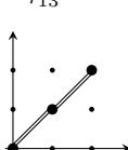
Here, we define the graph \(L^n_\sigma\) associated with a permutation \(\sigma\) below. Note that \(L^n_\sigma\) is always a simple graph and may contain cycles since a completely decreasing subsequence of length at least three in the permutation gives rise to a cycle in the graph \(L^n_\sigma\), as in Example 2.6, \(L^3_{\tau_{13}}\).

Definition 2.4. \[L_{\sigma}^{n} := \{\overline{c_{i\sigma(i)}c_{j\sigma(j)}} \subset \mathbb{R}^{2} \mid slope(\overline{c_{i\sigma(i)}c_{j\sigma(j)}}) > 0\}.\]

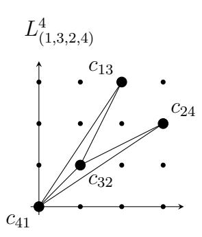
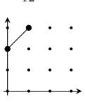
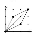
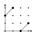
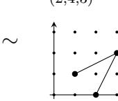
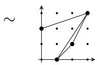
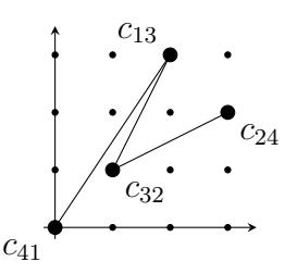
Example 2.5. For a full cyclic permutation \(\sigma=(1,3,2,4)\in S_4\), the associated graph \(L^4_\sigma\) is constructed as below:

\[\operatorname{inv}(\sigma) = \sharp \{(1,3), (2,3), (1,4), (2,4), (3,4)\} = \sharp \{\overline{c_{13}c_{32}}, \overline{c_{24}c_{32}}, \overline{c_{13}c_{41}}, \overline{c_{24}c_{41}}, \overline{c_{32}c_{41}}\} = 5.\]

In fact, the associated graph of any full cyclic permutation is always connected.

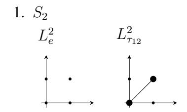
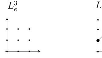
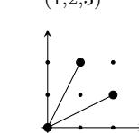
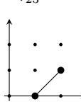
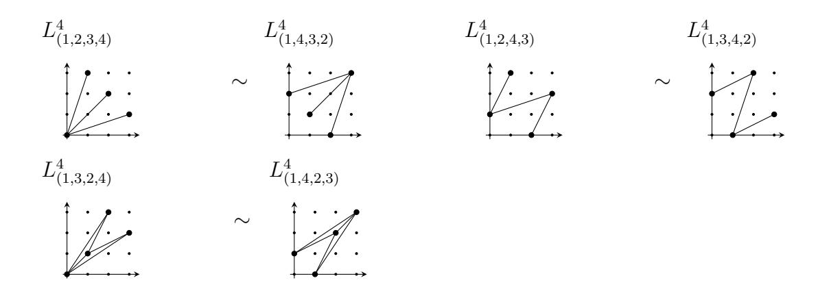
Example 2.6. For the symmetric groups of relatively small degree (n=2,3,4), the associated graphs are composed of paths, stars, and cycles: \(L^4_{(1,2,4,3)}\) is a path, \(L^4_{(1,2,3,4)}\) is a star, and \(L^4_{\tau_{13}\tau_{24}}\) is a cycle. The symbol \(\sim\) denotes an inverse permutation. If two permutations which are inverse to each other, then the associated graphs are isomorphic.

\[L^3_{(1,2,3)}\]

\[L_{\tau}^3\]

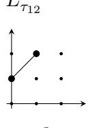
\[L^3_{(1,3,2)}\]

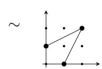
\[L^3_{\tau_{13}}\]

\[L^3_{\tau_{23}}\]

3. S⁴

L 4

\[L^4_{\tau_{14}\tau_{23}}\]

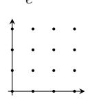
\[L_e^4\]

\[L^4_{\tau_{12}}\]

\[L_{\tau_{14}}^4\]

\[L_{\tau_{23}}^{4}\]

\[L_{\tau_{34}}^4\]

\[L^4_{\tau_{12}\tau_{34}}\]

\[L^4_{\tau_{13}\tau_{24}}\]

\[L^4_{(1,2,3)}\]

\[L^4_{(1,3,2)}\] L

∼

\[L^4_{(2,3,4)}\]

\[L^4_{(2,4,3)}\]

\[L^4_{(1,3,4)}\]

\[L^4_{(1,4,3)}\] L

\[L^4_{(1,2,4)}\]

\[L^4_{(1,4,2)}\]

3. Labeled Graphs with Edge Orderings

In order to study the graph theoretical properties of L n σ , we regard L n σ as an undirected graph. First we quickly review the basic and known facts in Graph Theory.

3.1. Labeled Graph

Let V = [n] and E be finite sets and γ be a map from E to a power set 2 V , and γ : E → 2 V satisfying |γ(e)| = 1 or |γ(e)| = 2 for an arbitrary element e ∈ E. The set (V, E, γ) is called an undirected graph G (it is just called a graph hereafter), and sets V and E are the vertex set and the edge set of G, respectively. A walk from x⁰ to x^r of a graph G is an alternating sequence of vertices and edges x0, e1, x1, e1, x2, . . . , xr−1, er, xr, in which each edge eⁱ is incident with the two points xi−1, xⁱ , and is expressed as x0x¹ · · · xr. When x⁰ = x^r in G, this walk is called a closed walk. The closed walk is called a cycle if each two vertices excluding x⁰ = x^r are different and any two edges are also different. It is a trail if all the edges are distinct, and a path if all the points (and necessarily all the edges) are distinct. A graph G is connected if a path exists between two arbitrary vertices on G. Furthermore, a connected graph without a cycle is called a tree, and a graph without cycles is called a forest. A subgraph H of G is a graph consisting of some vertices and edges in G. Let G¹ and G² be graphs. A mapping f from V (G1) to V (G2) is a homomorphism if f(i) and f(j) are adjacent in G² when i and j are adjacent in G1. Two graphs G¹ and G² are isomorphic (written G¹ ∼= G² ) if there exists a one-to-one correspondence between their vertices sets which preserve adjacency. The following results are known in Graph Theory.

Proposition 3.1 (Harary [3]). The following are the equivalent for a graph G with n vertices:

• (1) G is a tree.
• (2) Every two points of G are joined by a unique path.
• (3) G is connected and has n − 1 edges.

Definition 3.2. A graph G = (V, E, γ) is called a labeled graph if each edge eij in E with γ(eij ) = {i, j} corresponds to the transposition τ^eij = τij ∈ Sn. The vertices of a labeled graph are called the labeled vertices.

Dénes connected Linear Algebra and Graph Theory, and Moszkowski gave the exact bijection between them as follows:

Theorem 3.3 (Dénes [1], Moszkowski [7]). The number of representations of a given cyclic permutation of degree n by means of a product of a minimal number of transpositions is equal to the number of trees with n labeled vertices.

Remark 3.4. Eden and Schützenberger [2] obtained the number of associated cyclic permutations under the sorted equivalence for a given tree (see, Theorem 3.15).

3.2. Edge Orderings

In set theory, it follows from the axiom of choice that every set can be well-ordered. Therefore, we can define a well-ordering for a labeled graph. Let G be a graph and ω := (e1, e2, . . . , em), where eⁱ is an edge of G for 1 ≤ i ≤ m.

Definition 3.5. An edge ordering ω of a graph G is a linear order ≤^ω on the edge set E such that eⁱ ≤^ω e^j for i ≤ j.

Definition 3.6. Fⁿ := {(G, ≤ω) | G is a forest with n vertices, ≤^ω is an edge ordering of G}.

Definition 3.7. For any σ ∈ Sn, we define the labeled forest set

\[F_n(\sigma) := \{ (G, \leq_{\omega}) \in F_n \mid \tau_{e_m} \cdots \tau_{e_2} \tau_{e_1} = \sigma \},\]

where τ^ej is the transposition related to the edge e^j (see, Theorem 3.2).

We introduce a partial ordering among the edges of (G, ≤ω) in Fn(σ), and show that σ can be reconstructed by composing the transpositions according to the induced ordering.

Let σ be a permutation Sⁿ and σ = c^m · · · c2c¹ be the cycle decomposition of σ. For any k in [m] and i, j ∈ Supp(ck) (see, the definition of the support below), we define the distance d (σ) i (j) from i to j as follows:

Definition 3.8. \[d_i^{(\sigma)}(j) := \min\{r \in \mathbb{N} \mid j = \sigma^r(i)\}.\]

The order between two edges eij¹ and eij² sharing a common vertex i is defined by using the above distance d (σ) i as follows:

Definition 3.9. \[e_{ij_1} \leq_{\sigma} e_{ij_2}\] is defined by \(d_i^{(\sigma)}(j_1) \leq d_i^{(\sigma)}(j_2)\).

For two edges that do not share a vertex, the order is defined by requiring that the order between adjacent edges be preserved at each vertex along the path containing them. Let i0i¹ · · · i^r be a path on (G, ≤ω) in Fn(σ).

Definition 3.10. \[e_{i_0i_1} \leq_{\sigma} e_{i_{r-1}i_r}\] is defined by \(d_{i_{s+1}}^{(\sigma)}(i_s) \leq d_{i_{s+1}}^{(\sigma)}(i_{s+2}), (0 \leq s \leq r-2).\)

Since the graph is a forest, the path connecting the two edges is unique. Therefore, the order, whenever it exists, is uniquely determined.

Lemma 3.11. The order ≤^σ is a partial ordering on the set of all edges of (G, ≤ω) in Fn(σ).

Proof. It is clear from the definition of the order that the reflection and transition rules hold. Note that \(e_{ij} \leq_{\sigma} e_{kl}\) and \(e_{kl} \leq_{\sigma} e_{ij}\). The anti-symmetry law also holds since there exists only one path connecting any two vertices i and l in G by [3].

Let \(e_i\) and \(e_j\) be in E with i < j. A set \((G, \leq_{\sigma})\) is a well-ordered set if and only if \(e_j \leq e_i\) is not satisfied. Note that there are non-comparable parts in the well-ordered set; multiple well-orderings are possible. The well-ordering of \((G, \leq_{\sigma})\) can be regarded as the total-ordering. If the elements of \((G, \leq_{\sigma})\) are well-ordered, they are sorted as \(e_1, e_2, \ldots, e_m\) and this can be expressed as \(\leq_{\sigma} = (e_1, e_2, \ldots, e_m)\). We show that \(\sigma\) can be reconstructed by following the well-ordering \((G, \leq_{\sigma})\). First, we prepare Theorem 3.12.

Any permutation \(\sigma \in S_n\) is expressed as the product \(\tau_1 \tau_2 \cdots \tau_r\) of transpositions \(\tau_1, \tau_2, \ldots, \tau_r\), where the transposition product is taken from right to left of \(\tau_1 \tau_2 \cdots \tau_r\). The minimum value of the total number of transpositions denotes \(P_\sigma\). The length r cyclic permutation has a minimal transposition representation with \(P_\sigma = r - 1\). Let \(\sigma = (i_1, i_2, \ldots, i_r)\) be a cyclic permutation and denote the support of \(\sigma\), \(\mathrm{Supp}(\sigma) := \{i_1, i_2, \ldots, i_r\}\). Two cyclic permutations are prime to each other if their supports share no common parts. The decomposition into the product of the prime cyclic permutations is called a cycle decomposition. For the cycle decomposition \(\sigma = c_r \cdots c_2 c_1\) of a permutation \(\sigma\), \(P_\sigma = \sum_{i=1}^r P_{c_i}\).

Lemma 3.12. Let \(\tau\) be a transposition in the product of a minimal number of transpositions of a permutation \(\sigma\). Then there exists only one cyclic permutation c that appears in the cycle decomposition such that \(Supp(\tau) \subset Supp(c)\).

Proof. Let \(\sigma=c_r\cdots c_2c_1\) be the cycle decomposition for a permutation \(\sigma\in S_n\). Let \(\sigma=\tau_m\cdots \tau_2\tau_1\) be the minimum transposition representation. Then \(P_\sigma=m\). \(0=P_{\sigma^{-1}\sigma}=P_{\tau_1\tau_2\cdots\tau_mc_r}\). If \(\operatorname{Supp}(\tau_m)\cap\operatorname{Supp}(c_r)=\emptyset\), exchange \(\tau_m\) and \(c_r\). Then, there exists a cyclic permutation \(c_k\) such that \(\operatorname{Supp}(\tau_m)\cap\operatorname{Supp}(c_k)\neq\emptyset\). When \(\operatorname{Supp}(\tau_m)\subset\operatorname{Supp}(c_k)\), \(0=P_{\tau_1\tau_2\cdots\tau_{m-1}c_r}=P_{\tau_1\tau_2\cdots\tau_{m-1}c_r\cdots c_k\cdots c_2c_1}-1\) since \(P_{\tau_mc_k}=P_{c_k}-1\). When \(\operatorname{Supp}(\tau_m)\nsubseteq\operatorname{Supp}(c_k)\), \(0=P_{\tau_1\tau_2\cdots\tau_{m-1}c_r}=P_{\tau_1\tau_2\cdots\tau_{m-1}c_r\cdots c_k\cdots c_2c_1}+1\) since \(P_{\tau_mc_k}=P_{c_k}+1\). The same operation is applied to each \(\tau_i\). Let p be the number of the transpositions \(\tau_i\) with \(\operatorname{Supp}(\tau_i)\nsubseteq\operatorname{Supp}(c_k)\), and q be the number of the transpositions \(\tau_i\) with \(\operatorname{Supp}(\tau_i)\nsubseteq\operatorname{Supp}(c_k)\). It follows from \(0=P_\sigma-p+q\) and \(0\le p,q\le P_\sigma\). On the other hand, for the cycle decomposition \(\sigma=c_r\cdots c_2c_1\), we have \(0\le P_\sigma-\sum_{i=1}^r P_{c_i}+q\) is obtained since \(P_\sigma=\sum_{i=1}^r P_{c_i}\). From \(P_\sigma-p+q\le P_\sigma-\sum_{i=1}^r P_{c_i}+q\), we obtain \(\sum_{i=1}^r P_{c_i}\le p\). Thus, it follows from \(p\le P_\sigma\) that \(p=P_\sigma\) and q=0.

Lemma 3.13. Let \(\sigma = \tau_l \cdots \tau_2 \tau_1\) be the minimal transposition representation for any permutation \(\sigma \in S_n\) and let \(\tau_s = \tau_{ij}\) and \(\tau_t = \tau_{ik}\) for \(1 \leq s, t \leq l\). Then, s < t if and only if \(d_i^{(\sigma)}(j) < d_i^{(\sigma)}(k)\).

Proof. (Necessity) First, we show that if s < t, then \(d_i^{(\sigma)}(j) < d_i^{(\sigma)}(k)\). From Theorem 3.12, it is sufficient to show the case of the minimal transposition representation for a cyclic permutation. Hereafter, let \(\sigma \in S_n\) be a cyclic permutation.

Assume that \(\sigma = \tau_l \cdots \tau_t \cdots \tau_s \cdots \tau_1\) is the minimal transposition representation. The products from \(\tau_1\) to \(\tau_{t-1}\) are decomposed into prime cyclic permutations, this is set to \(\tau_{t-1} \cdots \tau_s \cdots \tau_1 = c_m \cdots c_2 c_1\), where, without losing generality, \(c_m\) can be a cyclic permutation \(\text{[rumus tidak dapat ditampilkan dengan baik — lihat PDF asli]}\)

ir), (r ≥ 2) including i, j. Then, τtc^m = τik(i, i1, . . . , j, . . . , ir) = (i, i1, . . . , j, . . . , ir, k). Hence, d (τtcm) i (j) < d(τtcm) i (k). For τtcm, it is shown that multiplying cp(1 ≤ p < m) from the right side of τtc^m or τq(t < q ≤ l) from the left side of τtc^m does not change the relationship in terms of the distance from i to k and j in the product.

First, we show that even if we multiply c^p (1 ≤ p < m) from the right side, the distance does not change. For the case where c1, . . . , c^m are all primes, the common part of c^p and τtc^m is just k. Let c^p = (k, j1, j2, . . . , j^rp ) and τtc^m = (i, i1, i2, . . . , j, . . . , ir, k), respectively. This product τtcmc^p = (i, i1, i2, . . . , j, . . . , ir, j1, j2, . . . , j^rp , k). It follows from d (τtcmcp) i (j) < d(τtcmcp) i (k) that d (τtcm···cp···c1) i (j) < d(τtcm···cp···c1) i (k).

Next, we show that, even if we multiply τtc^m · · · c^p · · · c¹ with τq,(t < q ≤ l) from the left side, the distance does not change. The case when the relative distances may change is multiplication τjk from the left side. However, three transpositions τij , τik, and τjk make a cycle, this is contradictory to the assumption that σ = τ^l · · · τ^t · · · τ^s · · · τ¹ is a cyclic permutation. Therefore, d (σ) i (j) < d (σ) i (k).

(Sufficiency) The sufficient condition can be shown in the similar way.

3.3. Reconstruction

It follows from Theorem 3.13 that we can reconstruct any permutation σ in Sⁿ by a wellordering of (G, ≤σ).

Theorem 3.14. Let (G, ≤ω) ∈ Fn(σ) be a labeled graph. Then the edge ordering ω = (e1, e2, . . . , em) is a well-ordering of (G, ≤σ).

Proof. From Theorem 3.12, the transpositions in the minimum transposition representation belong to the support of one cyclic permutation in the cycle decomposition. Therefore, transpositions belonging to the supports of different cycles in (G, ≤σ) cannot be compared: it does not become e^j ≤^σ eⁱ for i < j. It is sufficient to show that the sub-sequence comprising the edges corresponding to the minimum transposition representation of each cyclic permutation is well-ordered.

Let the minimum transposition representation of cyclic permutation c appearing in the cycle decomposition of σ be c = τ^ir · · · τⁱ² τi1 (1 ≤ i¹ < i² < · · · < i^r ≤ m). Let the edge corresponding to each transposition τⁱ be eⁱ ∈ (G, ≤σ).

Assume that, for 1 ≤ p < q ≤ ir, there exists e^q ≤^σ e^p . From this assumption and the definition of partial ordering ≤σ, we can take a sequence of line segments e^p0=^q ≤ e^p1 ≤ · · · ≤ e^pr=^p such that adjacent edges have a common point. It follows from Theorem 3.13 that there is p^s < ps+1 for an arbitrary 0 ≤ s ≤ r − 1. Hence, we have q < p, which is a contradiction. The minimal transposition representation c = τ^ir . . . τⁱ² τⁱ¹ gives the well-ordering of the corresponding edge sequence (eⁱ¹ , eⁱ² , . . . , e^ir ).

For a permutation σ ∈ Sn, let τ^m · · · τ2τ¹ and τ ′ ^m · · · τ ′ 2 τ ′ ¹ be two minimal transposition representations of σ.

Definition 3.15. The sorted equivalence τ^m · · · τ2τ^{1 s}∼ τ ′ ^m · · · τ ′ 2 τ ′ ¹ means that these two representations coincide by mutually sorting the transpositions.

Theorem 3.16. Let \((G, \leq_{\omega}) \in F_n(\sigma)\) be a labeled graph and \((e'_1, e'_2, \cdots, e'_m)\) be a well-ordering of \((G, \leq_{\sigma})\). Then \(\tau_m \cdots \tau_2 \tau_1 \stackrel{s}{\sim} \tau'_m \cdots \tau'_2 \tau'_1\), where is the edge corresponding to each transposition \(\tau_i\) be \(e_i \in (G, \leq_{\omega})\) and \(\tau'_i\) be \(e'_i \in (G, \leq_{\sigma})\).

Proof. Two edges which cannot be compared on \((G, \leq_{\sigma})\) do not have a common vertex from the definition of partially ordering \(\leq_{\sigma}\). Therefore, the corresponding transpositions are prime to each other. From the definition of the equivalence, we obtain \(\tau_m \cdots \tau_2 \tau_1 \stackrel{s}{\sim} \tau'_m \cdots \tau'_2 \tau'_1\).

4. Application

4.1. Minimal labeled graphs of \(L_{\sigma}^{n}\)

In this section, we treat \(L^n_\sigma\) as a graph by disregarding the coordinates from §2, i.e., the point \(c_{i\sigma(i)}\) in the graph \(L^n_\sigma\) as the vertex i and the line segment \(\overline{c_{i\sigma(i)}c_{j\sigma(j)}}\) as the edge \(e_{ij}=\{i,j\}\). Furthermore, the edge \(e_{ij}\) corresponds to the inversion-transposition [i,j] from the definition of \(L^n_\sigma\). From Theorem 3.12, it is enough to only consider the cyclic permutations. For this graph, we apply the edge ordering introduced in §3.2. In general, \(L^n_\sigma\) has a cycle. There the ordering \(\leq_\sigma\) is the pseudo-order, where the pseudo-order means that the partial ordering in which anti-symmetry is not satisfied.

We introduce a new notion "inversion-transposition". Let (k, l) be a transposition for \(k, l \in [n] = \{1, 2, ..., n\}\).

Definition 4.1. A transposition (k, l) is called an inversion-transposition [k, l] if (k, l) is an inversion.

This restriction to inversions is natural since inversion-transpositions correspond exactly to edges of \(L^n_\sigma\) and preserve the geometric structure of the graph.

Since there is no unique minimum inversion-transposition representation for a permutation \(\sigma \in S_n\), we must specify one minimal representation in order to define one of a minimal graph.

Definition 4.2. Let \(\sigma \in S_n\) be a permutation. Specify one minimal inversion-transposition's representation as \(\sigma = \tau_m \cdots \tau_2 \tau_1\), where m is the minimal number of inversion-transpositions of \(\sigma\). The minimal inversion-transposition graph \(\hat{L}^n_{\sigma=\tau_m\cdots\tau_2\tau_1}\) is defined as the labeled graph in which each edge corresponds to an inversion-transposition. We denote \(\{\hat{L}^n_\sigma\}\) as the set of minimal inversion-transposition graphs for a permutation \(\sigma \in S_n\). Therefore, the cardinality of \(\{\hat{L}^n_\sigma\}\) is equal to the number of the minimal inversion-transposition's representations for \(\sigma\).

In general, it is known that the permutation of an inversion number l is represented by the products of l transpositions. For the existence of \(\hat{L}_{\sigma=\tau_m\cdots\tau_2\tau_1}^n\), we show that any permutation is expressed by only inversion-transpositions.

Theorem 4.3. An arbitrary permutation \(\sigma \in S_n\) can be expressed by a product of a minimal number of inversion-transpositions.

Proof. Any permutation \(\sigma\) can be decomposed into the product of the prime cyclic permutations. Therefore, it is enough to consider the case of prime cyclic permutations. The proof proceeds by iteratively extracting inversion-transpositions corresponding to maximal elements, thereby reducing the cyclic permutation length step by step.

Let \(c = (i_1, i_2, \dots, i_r)\) be a prime cyclic permutation.

Step 1. Let c be reordered so that the rightmost element of c is the largest element: \(c = (i_1, i_2, \ldots, i_m)\), where \(i_m := \max\{i_1, i_2, \ldots, i_m\}\).

Step 2. For this \(i_m\), take out the elements which are inversions in order, and if an element which is not an inversion appears, back to Step1: for this \(i_m\), \((i_m,i_{m-1})\) is always an inversion since \(i_m\) is the largest element. Then we have \(c=(i_1,i_2,\ldots,i_{m-1})[i_{m-1},i_m]\), where \([i_{m-1},i_m]\) is an inversion-transposition. Next, check whether \((i_k,i_m)\), \((1 \le k \le m-2)\) is an inversion of c. Let \(i_{s_1}\) be the last element to be an inversion for \(i_m\); there exists \(s_1 \in \{2,\ldots,m-1\}\) such that \([i_{s_1},i_m]\) is an inversion, but \((i_{s_1-1},i_m)\) is not an inversion. Then, we have \(c=(i_1,i_2,\ldots,i_{s_1})[i_{m-1},i_m][i_{m-2},i_m]\cdots[i_{s_1},i_m]\).

Let \(c_{s_1} := (i_1, i_2, \ldots, i_{s_1})\). Subsequently, repeat the operation from Step1. Let \(c'_{s_1}\) be the reordered cyclic permutation of \(c_{s_1}\) such that the largest element of \(c_{s_1}\) is at the right end: \(c'_{s_1} := (i'_1, i'_2, \ldots, i'_{s_1})\), where \(i'_{s_1} := \max\{i'_1, i'_2, \ldots, i'_{s_1}\}\). Note that \(i'_{s_1} \neq i_{s_1}\) since \((i_{s_1-1}, i_m)\) is not an inversion. \((i'_{s_1-1}, i'_{s_1})\) is always an inversion; \(i'_{s_1-1} < i'_{s_1}\) since \(i'_{s_1} := \max\{i'_1, i'_2, \ldots, i'_{s_1}\}\). In the case of \(s_1 = 1\), we have \(c(i'_{s_1-1}) = c(i_{s_1}) = i_{s_1+1}\) and \(c(i'_{s_1}) = c(i_1) = i_2\). Since \([i_{s_1}, i_m]\) is an inversion, \(i_{s_1+1} = c(i_{s_1}) > c(i_m) = i_1 > i_2\). In case of \(s_1 \neq 1\), we have \(c(i'_{s_1-1}) = i'_{s_1}\) and \(c(i'_{s_1}) = i'_1\). Therefore, \(c(i'_{s_1-1}) = i'_{s_1} > i'_1 = c(i'_{s_1})\) since \(i'_{s_1} := \max\{i'_1, i'_2, \ldots, i'_{s_1}\}\).

The operation is continued until an element which is not an inversion appears. Let \(i'_{s_2}\) be the last element that becomes an inversion for \(i'_{s_1}\). Then, \(\text{[rumus tidak dapat ditampilkan dengan baik — lihat PDF asli]}\)

The operation ends with a finite number since the number of \(s_l (1 \le l \le m)\) is finite. Minimality is obvious since the elements are removed one by one.

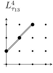
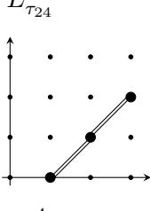
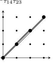
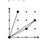
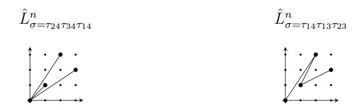
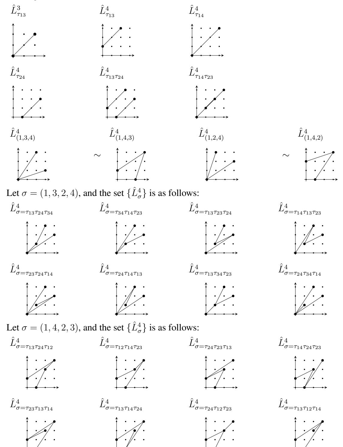
Example 4.4. A graph of \(\{\hat{L}_{\sigma}^n\}\) is determined only by inversion-transpositions, rather than by the order of the composition of them. Additionally, for a permutation, its graph may be different according to the minimum inversion-transposition's representation: \(\sigma=(1,3,2,4)\in S_4, \hat{L}_{\sigma=\tau_{24}\tau_{34}\tau_{14}}^n\) becomes a star graph sharing one point, and \(\hat{L}_{\sigma=\tau_{14}\tau_{13}\tau_{23}}^n\) becomes a path. These examples demonstrate the non-uniqueness of minimal inversion-transposition graphs and the structural diversity of such realizations.

Example 4.5. Consider \(\sigma \in S_n\) for n=2,3 and 4. Under sorted equivalence, the cardinality of \(\{\hat{L}_{\sigma}^n\}\) is 1 for n=2,5 for n=3, and 37 for n=4. The case in which the element of \(\{\hat{L}_{\sigma}^n\}\) differs

Remark 4.6. Let \(\sigma\) be a \(n \ (\geq 5)\) degree cyclic permutation. Under sorted equivalence, the cardinality of \(\{\hat{L}_{\sigma}^n\}\) is 192 if n=5, the cardinality is 3,180 if n=6, and the cardinality is 58,986 if

n=7. The connected labeled graph can be one of 3 types: paths, stars, and the composition of paths and stars.

4.2. Reconstructions by edge orderings of \(\hat{L}_{\sigma}^{n}\)

We apply the method developed in §3 in order to reconstruct the cyclic permutation from a given graph since \(\hat{L}_{\sigma=\pi_{o}}^{n}\) is the element of \(F_{n}(\sigma)\) from the definition.

Lemma 4.7. The order \(\leq_{\sigma}\) is a partial ordering on the set of all edges of \(\hat{L}_{\sigma}^{n}\).

The set comprising all the edges with semi-order in \(\hat{L}^n_{\sigma=\pi_\omega}\) is expressed as \((\hat{L}^n_{\sigma=\pi_\omega}, \leq_\sigma) = \{e_1, e_2, \ldots, e_m\}\). Let \(i, j \in (\hat{L}^n_\sigma, \leq)\) with i < j. If they are sorted so that it does not become \(l_j \leq_\sigma l_i\), this sorting is called \((\hat{L}^n_\sigma, \leq)\) well-ordering. As well-ordering allows the replacement of non-comparable parts, it is not necessarily the only one. When the elements of \((\hat{L}^n_\sigma, \leq_\sigma)\) are ordered so that they are sorted as \(l_m, \cdots, l_2, l_1\), this can be expressed as \(l_m \cdots l_2 l_1\). We show that \(\sigma\) can be reconstituted by ordering \((\hat{L}^n_\sigma, \leq_\sigma)\). It follows from Theorem 3.13 that we can reconstruct \(\sigma\) by well-ordering of \((\hat{L}^n_\sigma, \leq_\sigma)\).

Theorem 4.8. Let \(\sigma = \tau_m \cdots \tau_2 \tau_1\) be the minimal inversion- transposition representation of \(\sigma \in S_n\). Let \(l_i\) be the edge of \((\hat{L}^n_{\sigma = \tau_m \cdots \tau_2 \tau_1}, \leq_{\sigma})\) corresponding to the inversion-transposition \(\tau_i\). Then \((l_1, l_2, \cdots, l_m)\) is a well-ordering.

Theorem 4.9. For \(\sigma \in S_n\), let \(l_m \cdots l_2 l_1\) be a well-ordering of \((\hat{L}_{\sigma = \tau_m \cdots \tau_2 \tau_1}^n, \leq_{\sigma})\) and \(\tau_i'\) be the inversion-transposition corresponding to each edge \(l_i\). Then \(\tau_m \cdots \tau_2 \tau_1 \stackrel{s}{\sim} \tau_m' \cdots \tau_2' \tau_1'\).

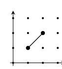
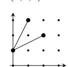
Example 4.10. For \(\sigma=(1,3,2,4)\in S_4\), consider the following graph \(\hat{L}_{\sigma}^4\). Each line segment \(l_{13}:=\overline{c_{13}c_{32}},\, l_{14}:=\overline{c_{13}c_{41}},\, l_{23}:=\overline{c_{24}c_{32}}\). From \(d_1^{(\sigma)}(3)=1\) and \(d_1^{(\sigma)}(4)=3\), we obtain \(l_{13}\leq_{\sigma}l_{14}\). From \(d_3^{(\sigma)}(2)=1\) and \(d_3^{(\sigma)}(1)=3\), we obtain \(l_{32}\leq_{\sigma}l_{31}\). Therefore we can arrange the line segments as \(l_{23}\leq_{\sigma}l_{13}\leq_{\sigma}l_{14}\). The minimal inversion-transposition representation corresponding to this well-ordering is \(\sigma=\tau_{14}\tau_{13}\tau_{23}\). In fact, the above graph can be obtained from this minimal inversion-transposition representation.

4.3. The relation between \(L^n_{\sigma}\) and \(\hat{L}^n_{\sigma}\)

In this section, we compare \(L^n_\sigma\) and \(\hat{L}^n_\sigma\) by using the concept of a spanning tree. A permutation \(\sigma \in S_n\) is called a full cyclic permutation if \(\sigma\) is a cyclic permutation of length n. Dénes [1] proved that the graph obtained from a full cyclic permutation is tree. Let G be a graph. A spanning subgraph is a subgraph containing all points of G. A spanning subgraph with no cycles is called a spanning forest, and a spanning tree if G is connected.

Remark 4.11. In the case of full cyclic permutations for n=2,3 and 4, the set of spanning trees of \(L^n_\sigma\) is isomorphic to \(\{\hat{L}^n_\sigma\}\). Then, by using the method in Section 4.2, we can reconstruct the permutation \(\sigma\) from one of \(\{\hat{L}^n_\sigma\}\). Otherwise, a spanning tree of \(L^n_\sigma\) does not necessarily coincide with one of \(\{\hat{L}^n_\sigma\}\): the permutation \(\sigma=\tau_{13}\tau_{24}\) for n=4 since \(\sigma=\tau_{13}\tau_{24}\) is of length 2.

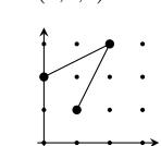
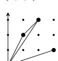
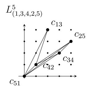
Remark 4.12. In the case of n=5, there exists a spanning tree that we can not reconstruct the permutation \(\sigma\): for \(\sigma=(1,3,4,2,5)\), the graph T on the right side below is one of spanning trees of \(L^5_{(1,3,4,2,5)}\), which is not contained in \(\{\hat{L}^5_{(1,3,4,2,5)}\}\); no matter how we take a product of the inversion-transpositions \(\tau_{23}\), \(\tau_{45}\), \(\tau_{25}\) and \(\tau_{15}\) corresponding for each edge on T, the permutation \(\sigma\) can not be reconstructed.

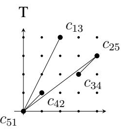
From the above Theorem 4.12, a spanning tree is not enough to reconstruct a given permutation. In order to obtain the necessary and sufficient conditions of the graph which can reconstruct a full cyclic permutation, we prepare some terminologies in Algebraic Graph Theory following Tsujie and Uchiumi [8], and Mohar and Thomassen [6].

Let \(G=(V,E,\gamma)\) be a graph. For a vertex \(v\in V\), let \(I_G(v):=\{e\in E\mid v\in\gamma(e)\}\) be the set of edges of G incident to a vertex v. When \(I_G(v):=\{e_1,e_2,\ldots,e_m\}\), a cyclic order \(\rho_v\) on \(I_G(v)\) is an equivalence class \([e_1,\ldots,e_m]\) of linear orders on \(I_G(v)\) obtained by identifying \((e_1,e_2,\ldots,e_m)\) with its circular shift \((e_2,\ldots,e_m,e_1)\). A rotation system of G is a collection \(\rho:=(\rho_v)_{v\in V}\) consisting of cyclic orders. We consider the pair \((G,\rho)\).

Let \(D_G := \{(e,v) \in E \times V \mid e \in I_G(v)\}\) be a set and the element is called a dart. A map \(\alpha: D_G \to D_G\) is defined by \(\alpha(e,v) := (e,u)\) for \(\gamma(e) = \{u,v\}\). A map \(\beta: D_G \to D_G\) is defined by \(\beta(e_i,v) := (\rho_v(e_i),v) = (e_{i+1},v)\), where \(\rho_v = [e_1,\ldots,e_m]\). Then, a bijection map \(\Phi: D_G \to D_G\) is defined by \(\Phi:= \beta \circ \alpha\).

We use the same representations as in Section 3.2. Given an edge ordering \(\omega=(e_1,e_2,\ldots,e_m)\), \(\pi_\omega:=\tau_{e_m}\cdots\tau_{e_1}.\) For a vertex \(v\in V, T_\omega(v):=\{e_i\in E\mid \tau_{e_i}\tau_{e_{i-1}}\cdots\tau_{e_2}\tau_{e_1}(v)\neq\tau_{e_{i-1}}\cdots\tau_{e_2}\tau_{e_1}(v)\}\) for \(i\geq 2, \tau_{e_0}(v)=v\) for \(\text{[rumus tidak dapat ditampilkan dengan baik — lihat PDF asli]}\) is the subset of E. When \(T_\omega(v)=\{e_{j_1},\ldots,e_{j_s}\}, (1\leq j_1<\cdots< j_s\leq m)\), we define a trail \(\omega_v:=(e_{j_1},\ldots,e_{j_s})\) from v to \(\pi_\omega(v)\). When a graph is a tree, any trail becomes a path since there are no cycles in the graph. A path of length r from r to r in a graph is a sequence of r+1 distinct vertices starting with r and ending with r, such that consecutive vertices are adjacent. The distance r distance r between two vertices r and r in r is the length of the shortest path joining them.

Theorem 4.13. Let \(\sigma \in S_n\) be a full cyclic permutation and T be a tree. Then the following are equivalent:

• (1) There exists an edge order \(\omega = (e_1, e_2, \dots, e_{n-1})\) of T such that \(\pi_{\omega} = \sigma\).
• (2) \(\sum_{v \in V} d_T(v, \sigma(v)) = 2(n-1)\), where \(d_T(v, \sigma(v))\) is the distance between v and \(\sigma(v)\) on T.

Proof. (1) \(\Rightarrow\) (2). From the assumption (1), let \(\omega\) be the edge ordering of G such that \(\pi_{\omega} = \sigma\). Then, we have \(d_T(v, \sigma(v)) = d_T(v, \pi_{\omega}(v))\). Moreover, since \(\omega_v\) is a trail on the tree \(T, d_T(v, \pi_{\omega}(v))\) is equal to the length of the trail \(\omega_v\). Hence, \(\sum_{v \in V} d_T(v, \sigma(v))\) is equal to the total number of edges of trails. It is enough to show that the total number of edges of trails is 2(n-1).

The cyclic order \(\rho_{\omega,v}\) is determined by \(\omega\) on each \(I_G(v)\) for a vertex \(v \in V\). Let \(\rho_\omega := (\rho_{\omega,v})_{v \in V}\) be a rotation system associated with \(\rho_\omega\). Consider this pair \((G,\rho_\omega)\). Let \(D_G := \{(e,v) \in E \times V \mid e \in I_G(v)\}\) be a set of darts, and the map \(\alpha:D_G \to D_G\) is defined by \(\alpha(e,v):=(e,u)\) for \(\gamma(e)=\{u,v\}\). The map \(\beta_\omega:D_G \to D_G\) is defined by \(\beta_\omega(e_i,v):=(\rho_{\omega,v}(e_i),v)=(e_{i+1},v)\), where \(\rho_{\omega,v}=[e_1,\ldots,e_m]\). Then, the map \(\Phi_\omega:D_G \to D_G\) is defined by \(\Phi_\omega:=\beta_\omega\circ\alpha\) associated with \(\omega\). Let the edge \(f_v\) be the smallest element of \(I_G(v)\) associated with \(\omega\), and \(O_\omega(f_v,v):=\{\Phi_\omega^k((f_v,v))\mid k\in\mathbb{Z}_{\geq 0}\}\) be an orbit of \(\Phi_\omega\) starting from a dart \((f_v,v)\). Then, there exists the minimum positive integer \(k_0\) satisfying \(\pi_\omega^{k_0}(v)=v\) and the set \(\{v,\pi_\omega(v),\ldots,\pi_\omega^{k_0-1}(v)\}=[n]\) and \(k_0=n\) since \(\sigma\) is a full cyclic permutation. Hence, the orbit \(O_\omega(f_v,v)\) becomes the connected closed walk connecting the endpoint of \(\omega_{\pi_\omega^{q-1}(v)}\) and the starting point of \(\omega_{\pi_\omega^q(v)}\) for \(0\leq q\leq k_0-1\) in order of trails \(\omega_v,\omega_{\pi_\omega(v)},\ldots,\omega_{\pi_\omega^{k_0-1}(v)}\). Therefore, the length of the orbit \(O_\omega(f_v,v)\) is equal to the total number of edges of trails, i.e., the cardinal number of edges of trails is 2(n-1).

Next, We show the contraposition of \((2) \Rightarrow (1)\). Suppose that \(\pi_{\omega} \neq \sigma\) for any edge ordering of G. Then, there exists a vertex \(v \in V\) such that \(\pi_{\omega}(v) \neq \sigma(v)\). For this v, the trail \(\omega_v\) does not coincide with the path from v to \(\sigma(v)\). Hence, the total number of all paths is not equal to 2(n-1).

This main theorem provides a complete graph-theoretic characterization of when a spanning tree reconstructs a full cyclic permutation.

Note that Theorem 4.13 is true for transpositions without restricting inversion-transpositions. By combining Theorem 3.3 and Theorem 4.3, the graph-theoretic properties that allow the cyclic permutation to be reconstructed from \(\hat{L}_{\sigma}^{n}\) are stated in Theorem 4.14.

Corollary 4.14. Let \(\sigma\) be a full cyclic permutation of \(S_n\) for any n. The set of spanning trees of \(L^n_{\sigma}\) satisfying the condition (2) of Theorem 4.13 is isomorphic to the set \(\{\hat{L}^n_{\sigma}\}\).

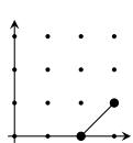
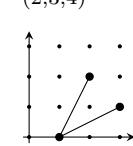
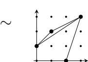
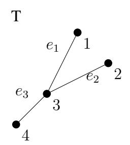
Remark 4.15. Let \(\sigma\) be a full cyclic permutation of \(S_n\) for any n. The graph that reconstructs \(\sigma\) does not necessarily come from \(L^n_{\sigma}\) or \(\hat{L}^n_{\sigma}\): for \(\sigma=(1,2,4,3)\), the tree T blow does not coincide with \(L^4_{\sigma}=\hat{L}^4_{\sigma}\). However, \(\sigma\) can be reconstructed with the edge ordering \(\omega=(e_1,e_2,e_3)\).

5. Conclusion

In this paper, we have introduced inversion-transpositions and have investigated their associated graphs and edge orderings, providing a graph-theoretic reconstruction criterion for full cyclic permutations. As a result, we have extended the classical results of Dénes by clarifying how geometric and order-theoretic structures on labeled graphs encode permutation data.

There are two natural directions for future research arising from this work. First, one may consider extending the framework to the case of non-cyclic permutations. Second, as mentioned in Theorem 4.6, the number of elements in the set \(\{\hat{L}^n_\sigma\}\) grows explosively, raising algorithmic problems concerning the enumeration of minimal inversion-transposition graphs. One possible approach is to investigate connections with the Cayley graphs of the corresponding groups associated with \(\hat{L}^n_\sigma\). Such a viewpoint may provide a more structural understanding and further deepen the scope of the inversion-transpositions framework.

Acknowledgement

The authors wish to thank Professor Yasuhide Numata for his useful contributions in the early stages of this research. This work has been supported in part by JSPS KAKENHI Grant Number JP23H05437.

References

• [1] J. Dénes, The representation of a permutation as the product of a minimal number of transpositions and its connection with the theory of graphs, Publications of the Mathematical Institute of the Hungarian Academy of Sciences, 4 (1959), 63-70.
• [2] M. Eden and M.P. Schützenberger, Remark on a theorem of Dénes, Publ. Math. Inst. Hungar. Acad. Sci., (1962), 353-355.
• [3] F. Harary, Graph Theory, Addison-Wesley Publishing Company, 1969.
• [4] A. Hurwitz, Über Riemannsche flächen mit gegebenen verzweigungspunkte, Mathematische Annalen, 39 (1891), 1-61.

• [5] A. Hurwitz, Über die anzahal der Reimannschen flächen mit gegebenen verzweigungspunkte, Mathematische Annalen, 55 (1902), 53-66.
• [6] B. Mohar and C. Thomassen, Graphs on Surfaces, Johns Hopkins University Press, 2001.
• [7] P. Moszkowski, A Solution to a problem of Dénes: a bijection between trees and factorizations of cyclic permutations, Europ. J. Combinatorics, 10 (1989), 13–16.
• [8] S. Tsujie and R. Uchiumi, Upper embeddability of graphs and products of transpositions associated with edges, Ars Mathematica Contemporanea, 25 (2025), no. 2, #P2.05.