Amir Barghia , Daryl DeFordb
aMathematics Program, Saint Michael's College, Colchester, VT
abarghi@smcvt.edu, ddeford@vassar.edu
In this paper we present enumerative results for Stirling numbers of the first kind for two graph products, the matched product and the m-star, using the combinatorial model of rearrangements. The kth Stirling number of the first kind for a simple graph G counts the number of ways to decompose G into exactly k vertex-disjoint cycles, including single vertices as 1-cycles, single edges as 2-cycles, and counting orientations for cycles of order three or higher. This naturally leads to the definition of the graphical factorial of G as the total number of such decompositions without any restrictions on the number of cycles involved. The matched product, motivated by a popular construction for modeling multiplex data, requires specifying a labeling of each component graph and naturally defines several families of graphs whose Stirling numbers of the first kind can be enumerated in terms of their component graphs. The m-star product of a graph G is defined as the join of G with the empty graph with m vertices. We compute the Stirling numbers of the first kind and factorials for the m-star of complete graphs, forests, and cycles, and we provide bounds for other families. The combinatorial proofs in the case of m-star products also motivate a generalization in terms of disjoint path decompositions of graphs, which provides another promising avenue of study.
Keywords: graph Stirling number of the first kind, graph factorial, matched product, cycle cover Mathematics Subject Classification : Primary 05C70; Secondary 05A15, 05A16, 05A19, 05A20, 05C30, 05C38, 05C45, 05C76. DOI: 10.5614/ejgta.2026.14.1.7
Received: 13 September 2023, Revised: 18 December 2025, Accepted: 18 January 2026.
bDepartment of Mathematics and Statistics, Vassar College, Poughkeepsie, NY
1. Introduction
1.1. Background
A cycle cover of a graph is a decomposition of the graph into cycles so that each vertex lies on exactly one cycle. One combinatorial interpretation of this problem is given by placing a marker on each vertex of the graph and then moving each marker along exactly one edge in such a way that each vertex again contains exactly one marker after the moves. This model is called the rearrange-ment problem following terminology introduced in [22, 26] for a given graph and enumerating these rearrangements across graph families leads to many fascinating combinatorial problems with formulas defined in terms of recurrence relations [6]. We also often consider the model where a marker is permitted to either move or stay in place, which can be modeled by adding a self-loop to every vertex in the graph, in which case we call this the rearrangement problem with stays. In particular, given that the number of rearrangements with stays on the path graph with n nodes is equal to the nth combinatorial Fibonacci number, many common graph families, including wheel graphs and generalizations, can be expressed in terms of combinations and products of Fibonacci numbers [5].
These decompositions have also been used to define graphical Stirling numbers of the first kind due to a natural recurrence relation given by considering decompositions into exactly k cycles. To provide context, we first discuss Stirling numbers of the second kind for graphs. Let G be a simple graph. The kth graphical Stirling number of the second kind for G, denoted by \({G \brace k}\), is the number of partitions of V(G) into k independent sets. The graphical Bell number for G is \(B_G = \sum_{k=0}^n {G \brace k}\), where n = |V(G)|. The graphical Stirling numbers of the second kind, explicitly introduced by Tomescu in 1971 [30], along with the Bell numbers for graphs, have been studied recently by Duncan and Peele [12], Duncan [11], Galvin and Tanh [17], Kereskényi-Balogh and Nyul [23], and Allagan and Serkan [1]. Galvin and Tanh [17] also lists a number of papers where Stirling numbers of the second kind for graphs have appeared earlier in the literature, even though in "various disguises." When G is the empty graph on n vertices, \(E_n\), we have \({G \brace k} = {n \brack k}\). Here, \({n \brack k}\) is the kth Stirling number of the second kind for n which is the number of ways of partitioning \([n] = \{1, \ldots, n\}\) into k parts.
Now let \(\begin{bmatrix} n \\ k \end{bmatrix}\) denote the kth (unsigned) Stirling number of the first kind, which counts the number of permutations of [n] into exactly k disjoint cycles. Moreover, we know that \(\sum_{k=0}^{n} {n \brack k} = n!\). Following the same line of thought, we define the graphical version of these numbers as follows: Let G be a simple graph. The kth graphical Stirling number of the first kind for G, denoted by \(\begin{bmatrix} G \\ k \end{bmatrix}\), is the number of partitions of G into exactly k directed cycles, where a single vertex is considered a 1-cycle, a single edge is considered a 2-cycle, and orientation for cycles of order three or higher matters. To prevent confusion, throughout the paper, by "cycle" we mean this more general definition, unless stated otherwise or obvious from the context. In the context of seating rearrangements with stays, a 1-cycle corresponded to a stay, a 2-cycle corresponds to a swap of the positions of two adjacent markers, and a cycle of length three or higher corresponds to a cyclic shift in the markers' positions. For a different formulation of the aforementioned definition of the kth graphical Stirling numbers of the first kind, see [2].
By analogy to graphical Bell numbers, the graphical factorial for G, denoted by G!, is defined as \(G! = \sum_{k=0}^{n} {G \brack k}\), where n is the order of the graph G. Also, it not hard to see that for a graph G with at least three vertices \({G \brack 1} = 2|\mathcal{H}(G)|\), where \(\mathcal{H}(G)\) is the set of distinct undirected Hamiltonian cycles of G. For results regarding the Stirling numbers of the first kind and graphical factorials for paths, cycles, complete bipartite graphs, wheels, and fans, see [2, 5, 6]. Some of the material, results, and derivations in Sections 1.2, 2, and 3 of this paper were originally presented in the appendix to DeFord's Ph.D. thesis [7].
It is noteworthy that graphical factorials are specifications of a general class of polynomials studied by Farrell [15]. Moreover, in a survey paper, Chiba and Yamashita [4] discussed the Stirling numbers of the first kind for graphs from an existential perspective, i.e., the conditions under which, for a fixed k, \(\begin{bmatrix} G \\ k \end{bmatrix} \neq 0\). More recently, an alternative definition for Stirling numbers of the first kind for graphs is introduced by Gonzales [18], which is motivated by an independent set formulation previously introduced by Engbers et al. [13] for Stirling numbers of the second kind for graphs. In this formulation by Gonzales, the analogy to the combinatorial Stirling numbers of first kind comes from evaluating on empty graphs, in the sense that the number of independent cycle decompositions with k cycles is equal to the regular Stirling number of the first kind. In our combinatorial model, the analogy is instead realized through complete graphs, since the number of rearrangements on the complete graph with k cycles is the regular Stirling number of the first kind.
1.2. Preliminaries
In this paper, we formulate a combinatorial graph product that generalizes constructions that originally arose in the context of multiplex networks. We then apply this product to construct families of graphs whose rearrangements can be computed efficiently. A multiplex or multi-layer network is a collection of networks, all defined on the same set of vertices, intended to capture different types of relationships between the objects or individuals being studied [24]. From a mathematical perspective, a multiplex can be described as an edge-colored graph, where the edges representing each distinct type of relationship are assigned a unique color.
There are several graph products whose usage has become standard in combinatorics. Examples include the Cartesian product, tensor product, lexicographical product, strong product, disjunctive product, and rooted product [19, 20]. Each of these products is defined for pairs of graphs, say G and H, and the vertex set of the product graph is all ordered pairs \((u,v) \in G \times H\). As in many areas of mathematics, it is frequently convenient to attempt to decompose a given graph into a product of smaller, simpler graphs and prove results about the properties of the combined object in terms of its components. A few examples of these products in network science include an analysis for multiple networks on a social network of computer scientists [25] and recent papers on Laplacian spectra of product networks [27, 28], which can be compared to similar analyses for the Erdős-Rényi model [10, 14]. Similarly, interesting combinatorial problems on graphs can be derived by focusing on extensions to different graph products [16, 29, 31].
A common feature of graph families whose rearrangements can be enumerated is the relative sparsity of edges in the graph, which makes the combinatorial analysis tractable. Many of the graph products mentioned above are dense in the sense that the number of edges grows like the product of the number of edges in the component graphs. In this paper, we focus on two product
models that generate relatively sparse graphs, and show that these lead to tractable enumerative results.
We begin by defining the formal graph product that generalizes a common construction of multiplex networks called the supra-adjacency matrix or matched sum. To this end, following a paper by DeFord and Pauls [8], we define the matched product of a sequence of layer graphs \((G_1, G_2, \ldots, G_k)\) with respect to a k vertex structure graph C as follows.
Definition 1.1. Suppose \(k \geq 2\). Let \(G_1, G_2, \ldots, G_k\) be an ordered list of graphs, each with n vertices and a common labeling of the vertices. Let C be a graph with k ordered vertices. The matched product \(\boxdot C(G_1, G_2, \ldots, G_k)\) is the graph with vertex set \(\bigcup V_i\), where \(V_i = V(G_i)\), and two vertices \(v_i^{\alpha}\) and \(v_j^{\beta}\) in \(\boxdot C(G_1, G_2, \ldots, G_k)\) are connected if and only if either
- \(c_{\alpha} \sim c_{\beta}\) and i = j, or
- \(\alpha = \beta\) and \(v_i^{\alpha} \sim v_i^{\alpha}\),
where \(c_{\alpha}\) and \(c_{\beta}\) are vertices in C and \(v_i^{\alpha}\) represents the copy of vertex i in \(G_{\alpha}\).
First, the matched product requires that the layer graphs have exactly the same number of vertices as well as a common labeling that allows us to identify the vertices that should be matched together. Secondly, the matched product is defined for multiple graphs but it is not naturally associative.
A convenient feature of this generalization is that three of the standard multiplex models can be expressed efficiently in this notation with the matched sum \(\Box K_k(G_1, G_2, \ldots, G_k)\), disjoint layers \(\Box E_k(G_1, G_2, \ldots, G_k)\), and temporal matched sum \(\Box P_k(G_1, G_2, \ldots, G_k)\) each having a compact representation. Throughout this paper, \(P_k\) is the path graph on k vertices and \(S_k\) is the star graph on k+1 vertices. For the star graph, the non-leaf vertex will be called the root. Thus, the matched product provides a general framework for describing a wide range of multiplex constructions. For more descriptions and analysis of these models, see papers by DeFord and Pauls [7, 8, 9]. Throughout this paper, the chosen labeling for each example will be made clear in context or described with a figure. Moreover, \(C_k\) is the cycle graph of order k.
The other product we focus on in this paper is the join of two graphs: The join of two simple graphs G and H, denoted by \(G \bowtie H\), is the graph whose vertex set is \(V(G) \cup V(H)\) and whose edge set is \(E(G) \cup E(H) \cup \{uv \mid u \in G, v \in H\}\). Now let us assume that G has n vertices and H is \(E_m\) the empty graph of m vertices. We define the m-star graph of G as \(S_m(G) = G \bowtie E_m\). For example, the complete bipartite graph \(K_{n,m}\) is the m-star graph of \(E_n\).
Throughout this paper, we denote the falling factorial power \(x(x-1)\cdots(x-k+1)\) by \(x^{\underline{k}}\), where \(x\in\mathbb{R}\) and \(k\in\mathbb{N}\). Finally, we use Iverson bracket which is defined as
\[[P] = \begin{cases} 1, & \text{if } P \text{ is true,} \\ 0, & \text{otherwise.} \end{cases}\]
2. The Matched Product
We begin our analysis by recording some basic counting information about the matched product, including the number of additional edges that are added in this construction, compared to the disjoint layers.
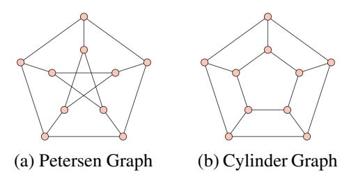
Figure 1: An example of the matched product construction. Plots (a) and (b) show non-isomorphic orderings of \(\Box P_2(C_5, C_5)\).
Lemma 2.1. Suppose n is a positive integer. Let |V(C)| = k, \(|V(G_i)| = n\) for all \(1 \le i \le k\). Then, the matched product \(\square C(G_1, \ldots, G_n)\) is a graph with nk vertices and \(|E(C)|n + \sum_{i=1}^k |E(G_i)|\) edges. In particular, in the case of the matched sum, where \(C = K_k\) there are \(\binom{k}{2}n\) additional inter-layer edges.
Although this is a simple result, the consequences of adding this many edges to the network model have significant impacts on practical applications of the matched sum. In cases where the component networks are sparse, as in most social networks, it is possible that inter-layer edges have been added in this construction process than were present in the original layer networks. For our use in this paper, this sparsity of edges between the layers is an asset of the model, allowing us to use combinatorial methods to enumerate rearrangements.
We next note that the ordering of the vertices has significant consequences for the matched product. Figure 1 highlights that graphs with isomorphic layer graphs and structure graph need not be isomorphic by showing the Petersen graph and the "5-cylinder" as two non-isomorphic examples of \(\boxdot P_2(C_5, C_5)\) formed with different labelings. Other examples of common graphs that can be written with this product include the hypergraph as the iterated \(P_2\) matched product \(\boxdot P_2(\boxdot P_2, \cdots (\boxdot P_2(P_2, P_2)) \cdots)\) and the grid graphs as \(\boxdot P_m(P_n, P_n, \ldots, P_n)\). This ability to decompose well-known families of graphs into component layers will prove useful for enumerating graph rearrangements below.
Although motivated by the matched sum construction for networks, the examples above demonstrate that this product also realizes several previously studied graph products as special cases. We record these relations in the following result, noting that this allows us to apply results derived for these products, to the corresponding matched product forms.
Proposition 2.1. There are labelings of the graphs below such that the following hold:
- 1. The Cartesian product of G and H can be represented by \(\boxdot H(G, G, \ldots, G)\).
- 2. The rooted product of G and H can be represented by \(\Box H(G, E_n, E_n, \dots, E_n)\).
- 3. The hierarchical product of G and H with subset \(\{a_i\} \subseteq H\) can be represented by \(\boxdot H(G_1, G_2, if i \in \{a_i\})\).
\[G_2, \ldots, G_k\]), where \(G_i = \begin{cases} G, & \text{if } i \in \{a_i\}, \\ E_n, & \text{otherwise.} \end{cases}\)
Proof.
- 1. Two vertices (u, v) and (w, x) in the Cartesian product are connected if and only if u ∼ w or v ∼ x. Note that the Cartesian condition is equivalent to the construction of |V (G)| copies of H and connecting all copies of a given label according to the connections in G, which is equivalent to ⊡ H(G, G, . . . , G).
- 2. The rooted product is constructed by fixing a root vertex in H and considering |V (G)| copies of H with the roots connected according to the connections in G. In
\[\Box H(G, E_n, E_n, \ldots, E_n),\]
we have a single copy of G and then n copies of H joined at the root by the connections in G exactly as desired. In general, filling the list (G1, G2, . . . , Gk) with copies of En simply gives that many disjoint copies of the graph H.
3. The hierarchical product is a more recent invention, introduced by Barriére et al. [3] and studied as a network model by Skardal [28]. Here the product is taken with respect to two graphs G and H, as well as a subset of the vertices of H. The construction begins with the rooted product of G and H but the copies of H that are associated with the subset are connected according to the edges of G, instead of remaining empty. This is exactly the construction stated in the theorem in terms of the matched product.
3. Rearrangements and Derangements of Labelings
In addition to the Stirling numbers of the first kind for graphs, we have the following definition that we use in this paper: let -G j denote the number of decompositions of a given graph G into j disjoint cycles where 1-cycles are not allowed—these are rearrangements without fixed points, i.e., derangements. The total number of derangement is denoted by G! = P k -G j , similar to the definition of graphical factorial we saw earlier.
Throughout our combinatorial discussion, we mostly focus on applications to the matched products of two graphs with P2 as the structure graph. Even this simple subcase leads to several interesting observations and applications and indeed many of the rearrangement problems considered by Barghi [2] and DeFord [6] can be constructed using the matched product. For example, Theorem 9 in DeFord's paper [6] concerns ⊡ P2(G, G) for a bipartite graph G while Example 10 and 11 in the same paper explicitly compute
\[\sum_{k} \begin{bmatrix} \boxdot P_2(C_n, C_n) \\ k \end{bmatrix} \text{ and } \sum_{k} \overline{\begin{bmatrix} \boxdot P_2(C_n, C_n) \\ k \end{bmatrix}}.\]
Before enumerating some classes of rearrangements, we record a preliminary observations about the properties of the matched products of two graphs with P2 as the structure graph. Considering the combinatorial interpretation of rearrangements often leads to natural questions about distinguished paths and cycles in the graph as well as questions of planarity, as every planar graph admits a Pfaffian orientation, which in turn can allow for an efficient computation of the number of rearrangements. As we saw above in Figure 1, in the case of the Petersen Graph and the 5-cylinder, the labeling of the vertices in each copy can have significant consequences on the properties of the
constructed graph. This same example shows that planarity is not a preserved property of the matched product, even with two layers, at least for all labelings [7]. This suggests a natural extension to enumerating the labelings that do preserve a fixed property, which we suggest as a potential avenue for future work.
Given this new graph product and a desire to compute rearrangements, we begin with the simple case of ⊡ P2(G, En) for an arbitrary graph G. We call these the "comb" graphs since they consist of a single edge sticking up from each vertex.
Proposition 3.1. Let G be an arbitrary graph on n ≥ 1 vertices. Then,
\[\overline{\begin{bmatrix} \boxdot P_2(G, E_k) \\ j \end{bmatrix}} = \begin{cases} 1, & \text{when } j = n, \\ 0, & \text{otherwise.} \end{cases}\]
And
\[\begin{bmatrix} \boxdot P_2(G, E_k) \\ j \end{bmatrix} = \sum_{U \subset G, |U| < j} \begin{bmatrix} G \setminus U \\ j \end{bmatrix}.\]
Proof. The unique rearrangement in
\[\begin{bmatrix} \boxdot P_2(G, E_k) \\ n \end{bmatrix}\]
connects every vertex in G to the corresponding vertices in the empty graph, giving G! = 1. For
\[\begin{bmatrix} \boxdot P_2(G, E_k) \\ j \end{bmatrix},\]
we select a subset of vertices to pair with the empty vertices and rearrange the remaining vertices in G.
We next compute some specific examples of rearrangements on comb graphs and then show how they can be combined for more complex enumerations. For each of these examples, we report the factorials, while the individual rearrangement numbers can be recovered from the proofs if desired. We denote the well-known Pell numbers by Ln, with L0 = 1, L1 = 2, and Ln = 2Ln−1 + Ln−2 (listed as the sequence A000129 in OEIS [21]). Throughout this paper, when applying the rearrangement model, we identify each marker by the name or label of the vertex on which it was originally placed.
Proposition 3.2. Let n be a positive integer. Then, we have
- 1. ⊡ P2(En, En)! = 2n ;
- 2. ⊡ P2(Pn, En)! = Ln;
- 3. ⊡ P2(Sn, En)! = 2n+1 + n2 n ;
- 4. ⊡ P2(Cn, En)! = 2 · (⊡ P2(Pn−1, En−1)! + ⊡ P2(Pn−2, En−2)! + 2);
- 5. ⊡ P2(Kn, En)! = P ℓ n ℓ (n − ℓ)!.
Figure 2: This figure shows the star graph on eight vertices (a) as well as the product graph \(P_2(S_8, P_9)\) where the root of the star is connected to a leaf of the path (b).
Proof.
- 1. The graph \(\Box P_2(E_n, E_n)\) consists of n copies of \(P_2\), each of which may have the two adjacent vertices swap positions or remain in place giving \(\Box P_2(E_n, E_n)! = 2^n\).
- 2. We note that \(\boxdot P_2(P_1, E_1)! = P_2! = 2\) and \(\boxdot P_2(P_2, E_2)! = P_3! = 5\). Working recursively, we consider computing \(\boxdot P_2(P_n, E_n)!\) from \(\boxdot P_2(P_{n-1}, E_{n-1})!\) by conditioning on the behavior of the two added vertices. If these adjacent vertices both remain in place or swap positions with each other, we are left with \(\boxdot P_2(P_{n-1}, E_{n-1})!\) ways to rearrange the remaining vertices. Otherwise, the new path vertex must swap places with the (n-1)st path vertex and the two corresponding E vertices must remain in place, leaving \(\boxdot P_2(P_{n-2}, E_{n-2})!\) ways to rearrange the remaining vertices. As this is the recurrence for Pell numbers and our initial conditions are equal to E1 and E2, we are done.
- 3. We condition on the behavior of the root of \(S_n\). If the root remains in place or swaps places with the corresponding adjacent E vertex, the remaining graph is \(\Box P_2(E_n, E_n)!\) which we enumerated in part 1 as \(2^n\). If the root swaps with one of its adjacent leaves, the remaining graph is \(\Box P_2(E_n, E_n)\) together with a disconnected vertex. As there are n leaves to swap with, we are done.
- 4. We condition on the behavior of an arbitrary distinguished vertex, x, from the cycle. If x remains in place or swaps with the corresponding adjacent vertex in \(E_n\) the remaining graph is \(\Box P_2(P_{n-1}, E_{n-1})\), enumerated in part 2. Similarly, if x swaps places with either of its neighbors around the cycle, we are left with \(\Box P_2(P_{n-2}, E_{n-2})\). Finally, the entire cycle can be traversed in either direction with all of the \(E_n\) vertices remaining in place.
- 5. For this example it is most natural to condition on the number of vertices in the \(K_n\) that do not swap with the corresponding adjacent vertex in \(E_n\). This leads us to select k of these vertices, in \(\binom{n}{k}\) many ways, which can be arranged in k! ways. Summing over all values of k gives the result.
This collection of results highlights many of the standard techniques that are used for enumerating rearrangements, including building up to more complex structures from simpler ones, and arguing recursively as well as directly. We next compute the two sets of rearrangements for the \(\boxdot P_2(S_n, P_n)\) where the root of the star is connected to a leaf of the path as in Figure 2. It is interesting to note that the products \(\boxdot P_2(P_n, S_n)\) and \(\boxdot P_2(S_n, S_n)\) are planar for all labelings as
the leaf vertices can be rearranged in any embedding. A related question for future work is determining choices of G and H such that \(\boxdot P_2(G,H)\) are isomorphic for all labelings. An example with this property is given by \(\boxdot P_2(S_n,C_n)\). Note that although \(\boxdot P_2(P_n,S_n)\) and \(\boxdot P_2(S_n,S_n)\) are always planar, they are not isomorphic for all labelings because of the non-leaf in \(S_n\) and the endpoints of \(P_n\).
Proposition 3.3. Let n be an integer greater than 2. Then, if the label of the root of the star is the same as one of the leaves of the path, we have \(\overline{ \boxdot P_2(S_n, P_n)!} = 4\) and
\[\Box P_2(S_{n+1}, P_{n+1})! = 2 \Box P_2(S_n, P_n)! + \Box P_2(S_{n-1}, P_{n-1})! + L_n + 3L_{n-1} + 2L_{n-2}\] \[+2 \sum_{n=1}^{n} (L_{n-1} + L_{n-2}) + 2.\]
Proof. In order to simplify this proof, we provide some terminology for distinguishing the vertices in the product. Let r be the root of the star graph. We label the vertex in \(P_n\) adjacent to r in \(\boxdot P_2(S_n, P_n)\) with \(p_0\) and index the remaining vertices in \(P_n\) sequentially starting from \(p_0\) by \(\{p_1, p_2, \ldots, p_{n-1}\}\). The leaf in the star connected to \(p_j\) will be denoted by \(\ell_j\), for \(1 \le j \le n\).
For derangements, we can discover the four decompositions by conditioning on r. The root can swap places with either \(p_0\) or \(\ell_1\). In either case, the remaining vertices must be paired in the unique perfect matching. Alternatively, these four vertices may form a cycle \(p_0, \ell_1, p_1, r\), in either direction, leaving the remaining vertices to pair in a matching.
We enumerate the rearrangements in two ways: first recursively and then give a direct proof in the Appendix. The recursive formula is the one stated in the proposition.
Recursive: We condition on the behavior of the newly added vertices \(p_{n+1}\) and \(\ell_{n+1}\). If the new vertices swap places with each other or remain in place, we are left with all of the arrangements on the original graph \(\Box P_2(S_n, P_n)\). If \(\ell_{n+1}\) remains in place and \(p_{n+1}\) swaps places with \(p_n\), either \(\ell_n\) also remains and we have \(\Box P_2(S_{n-1}, P_{n-1})\), or the root swaps with \(\ell_n\), and we have \(L_{n-1} + L_{n-2}\) rearrangements, depending on whether \(p_0\) remains or swaps with \(p_1\) respectively. As this type of argument reoccurs, we highlight the fact that once the behavior of the root has been decided, we are usually left with subgraphs equivalent to \(\Box P_2(P_m, E_m)\), for some m, to count the remaining rearrangements. We note that since the root is now determined, either \(p_0\) remains in place, leaving \(\Box P_2(P_m, E_m)\), or it swaps places with \(p_1\), forcing \(\ell_1\) to remain in place and leaving \(\Box P_2(P_{m-1}, E_{m-1})\).
We next enumerate the cases where \(\ell_{n+1}\) swaps places with r. If \(p_0\) and \(p_{n+1}\) remain in place, there are \(L_n\) ways to rearrange the remaining \(\boxdot P_2(P_n, E_n)\), since if \(p_0\) swaps with \(p_1\) or \(p_{n+1}\) swaps with \(p_n\), we have \(L_{n-1}\), and if both \(p_0\) swaps with \(p_1\) and \(p_{n+1}\) swaps with \(p_n\) we have \(L_{n-2}\) rearrangements. Next, there are cycles with one of \(\ell_{n+1}\) going to r or vice versa. For each of these, we can choose an index j to represent the other leaf that is connected to r, leaving \(L_{j-1} + L_{j-2}\) rearrangements depending on the behavior of \(p_0\). Finally, we have the two cycles formed through r and the new vertices.
We conclude this section with some numerical computations on matched products where the graphs are isomorphic regardless of labeling. The rearrangements are displayed in Table 1. We
Table 1: This table reports the number of rearrangements of several natural matched products whose structure are not determined by the labeling of the vertices on the layer graphs. None of these sequences have appeared previously in the OEIS [21]
| n | \[\overline{\boxdot P_2(C_n,S_n)!}\] | \[\overline{\boxdot P_2(K_n,S_n)!}\] | \[\boxed{ \boxdot P_2(P_n, K_n)!}\] | \[\overline{\boxdot P_2(C_n,K_n)!}\] | ||
|---|---|---|---|---|---|---|
| 2 | 9 | 48 | 4 | 9 | 4 | 9 |
| 3 | 49 | 293 | 9 | 48 | 20 | 82 |
| 4 | 140 | 2022 | 49 | 345 | 121 | 577 |
| 5 | 394 | 15657 | 216 | 2994 | 589 | 4876 |
| 6 | 1093 | 135044 | 1773 | 30957 | 4820 | 49789 |
| 7 | 2986 | 1287813 | 12113 | 369132 | 35293 | 587182 |
| 8 | 8056 | 13480938 | 128036 | 4996761 | 365633 | 7887553 |
| 9 | 21504 | 153879977 | 1172341 | 75625710 | 3525212 | 118596664 |
| 10 | 56889 | 1903771512 | 14885241 | 1265833149 | 43894725 | 1974218701 |
note that the formulas for \(\Box P_2(C_n, S_n)! = 9\) and \(\Box P_2(K_n, S_n)! = (n+1)^2\) can be proved in a similar method to the one we employed on the star graphs in Proposition 3.3.
4. Rearrangements of Stars of Graphs
One case of matched products is \(\Box P_2(G, E_n)\), which we called comb graphs. At a different extreme, we have star graphs \(S_n(G) = G \bowtie E_n\), where each vertex in \(E_n\) is adjacent to all the vertices in G. To understand \(S_n(G)\) better, since we do not need the restriction that all the layers have the same order, we look at \(S_m(G)\), where m can be different than n. This has the advantage that it allows us to find recurrence relations for \({S_m(G) \brack k}\) and \(S_m(G)\)!, where G is either a complete graph, forest, or cycle, allowing us to find upper and lower bounds for these numbers. We first state some properties of \({S_m(G) \brack k}\) and \(S_m(G)\)! when G is any graph and then focus on complete graphs and forests.
Definition 4.1. Let G be a graph with n vertices. We denote the cardinality of the set of all partitions of G into j vertex-disjoint directed and ordered paths by \(\binom{G}{j}\), where we call each part in of one these partitions a partitioning directed path in G. Clearly, \(\binom{G}{n} = n!\), and \(\binom{G}{m} = 0\) when m > n.
Theorem 4.1. Let G be a graph with \(n \geq 2\) vertices. If \(m \leq n\), then \(\binom{S_m(G)}{1} = (m-1)! \binom{G}{m}\); otherwise, \(\binom{S_m(G)}{1} = 0\).
Proof. We know that in every directed Hamiltonian cycle C of \(S_m(G)\), for every vertex in \(E_m\) visited by C, we visit exactly one vertex in G afterwards. All the vertices in G visited by C are distinct from each other, which explains the condition \(m \leq n\). Also, this is the reason why we are looking at partitioning G into exactly m paths: If we remove the vertices in \(E_m\), as we traverse C, we are left with m vertex-disjoint directed and ordered paths in G.
Now we construct a directed Hamiltonian cycle as follows: Let π = π1, . . . , πm be a partition of G into exactly m vertex-disjoint directed and ordered paths, and let µ = µ1, . . . , µm be a rearrangement of the vertices in Em. Use µ1 to connect the first vertex in π1 to the last vertex in πm. Then connect πi+1 to πi using µi+1 so that the leftmost vertex in πi+1 is connected with the rightmost vertex in πi via µi . Clearly, this process creates an orientation, but each cycle thus created has been overcounted by a factor of m due to rotation; hence, we have (m − 1)! G m possibilities.
Theorem 4.2. Let G be a graph with n ≥ 2 vertices. If m ≤ n, then
\[\begin{bmatrix} S_m(G) \\ 2 \end{bmatrix} = m \begin{bmatrix} S_{m-1}(G) \\ 1 \end{bmatrix} + \begin{bmatrix} m \\ 2 \end{bmatrix} \begin{pmatrix} G \\ m \end{pmatrix};\]
otherwise, -Sm(G) 2 = 0.
Proof. If one of the vertices in Em is in a 1-cycle, then they rest of the graph which is isomorphic to Sm−1(G) must form a single cycle. This gives us the first term on the right-hand side. The other possibility is that all the vertices in Em are in cycles involving vertices in G. In this case, we partition the vertices in Em into two cyclic parts, (v1, . . . , vi) and (u1, . . . , um−i). Next, we partition G into m vertex-disjoint directed and ordered paths π1, . . . , πm. The two cycles in Sm(G) are C1 = v1, π1, . . . , vi , πi and C2 = u1, πi+1, . . . , um−i , πm. This justifies the second term on the right-hand side.
For the material discussed in the next section, we need the following:
Proposition 4.1. If \[n \ge 1\], then \(\binom{K_n}{j} = n! \binom{n-1}{j-1}\) (listed as the sequence A156992 in OEIS [21]).
Proof. We first rearrange the vertices of Kn in n! ways. With the first path starting with the first vertex in the rearrangement, we need to mark where each of the remaining j − 1 paths start along the rearrangement, which can be in n−1 j−1 ways.
Using Theorem 4.1 and Proposition 4.1, we have the following:
Proposition 4.2. Let n ≥ 1. If 1 ≤ m ≤ n, then -Sm(Kn) 1 = (n − 1)!n m; otherwise, -Sm(Kn) 1 is equal to zero.
We finish this section with the following result whose proof is obvious:
Theorem 4.3. Let n, m ≥ 1. If G is a graph of order n, then
\[K_{n,m}! \le S_m(G)! \le K_{n+m}!.\]
Remark 4.1. Deford [6] proved that
\[K_{n,m}! = \sum_{i=0}^{\min\{m,n\}} m^{i} n^{i}.\]
The values of Km,n! are listed as the sequence A099597 in OEIS [21]. Moreover, the values of Km,n! when m = n are listed as the sequence A006040 in OEIS [21].
5. Rearrangements of Stars of Complete Graphs
We denote the m-star of a complete graph on n vertices by \(S_{n,m} = S_m(K_n)\). It is also easy to check that for \(S_{1,m}\) and \(S_{2,m}\), we have the following results:
Proposition 5.1. Let \(m \in \mathbb{N}\). For \(k \notin \{m, m+1\}\), \(\begin{bmatrix} S_{1,m} \\ k \end{bmatrix} = 0\), and \(\begin{bmatrix} S_{1,m} \\ m+1 \end{bmatrix} = 1\) and \(\begin{bmatrix} S_{1,m} \\ m \end{bmatrix} = m\). Moreover, \(S_{1,m}! = m+1\).
Proposition 5.2. Let \(m \in \mathbb{N}\). For \(k \notin \{m-1, m, m+1, m+2\}\), \({S_{2,m} \brack k} = 0\), and \({S_{2,m} \brack m+1} = 2m+1\), \({S_{2,m} \brack m} = 2m+m(m-1)\), and \({S_{2,m} \brack m-1} = m(m-1)\). Moreover, \(S_{2,m}! = 2(m^2+m+1)\).
We include similar simple results for derangments of stars in Appendix Appendix B. Knowing the value of \(\begin{bmatrix} S_{n,m} \\ 1 \end{bmatrix}\) from Proposition 4.2 and that \(\begin{bmatrix} S_{n,m} \\ n+m \end{bmatrix} = 1\), we find \(\begin{bmatrix} S_{n,m} \\ k \end{bmatrix}\) for \(2 \le k < n+m\).
Theorem 5.1. Let \(n, m \in \mathbb{N}\) with \(m \leq n\). Then, for \(2 \leq k < n + m\),
\[\begin{bmatrix} S_{n,m} \\ k \end{bmatrix} = \begin{bmatrix} n \\ k-m \end{bmatrix} + \sum_{i=1}^{m} \sum_{j=1}^{n} \sum_{l=0}^{n-1} {m \choose i} \begin{bmatrix} n-j \\ l \end{bmatrix} j! {j \choose i-1} \begin{bmatrix} i \\ k-(m-i+l) \end{bmatrix}.\]
Proof. We prove this theorem combinatorially by showing that
\[\begin{bmatrix} S_{n,m} \\ k \end{bmatrix} = \begin{bmatrix} n \\ k-m \end{bmatrix} + \sum_{i=1}^{m} \sum_{j=i}^{n} \sum_{l\geq 0} {m \choose i} {n-j \brack l} {K_j \brack i} {i \brack k-(m-i+l)},\]
and then applying Proposition Appendix B.1.
We first choose m-i vertices in \(E_m\) to be 1-cycles, with the remaining vertices in \(E_m\) being in cycles of order two or higher. Removing these 1-cycles leaves a graph G isomorphic to \(S_{n,i}\). When i=0, we get the first term. As a result, we may assume that i>0. Denote the induced subgraphs \(G\cap E_m\simeq E_i\) and \(G\cap K_n\simeq K_n\) by \(G_1\) and \(G_2\), respectively. Now split \(G_2\) into two disjoint induced subgraphs: Let \(H_1\) be the induced subgraph of \(G_2\) consisting of vertices that are part of cycles with vertices in \(G_1\), and let \(H_2\) be the induced subgraph of \(G_2\) whose vertices are in \(V(G_2)-V(H_1)\). It is not difficult to see that both \(H_1\) and \(H_2\) are cliques in \(G_2\).
Suppose the vertices in \(G_1\) are labeled \(\mu_1, \ldots, \mu_i\). Let C be a cycle of order two or higher in \(S_{n,m}\) that visits \(V(G_1)\), and let \(v \in V(C) \cap V(G_1)\). Starting with v and traversing C, after each visit to a directed partitioning path in \(H_1\), we visit a vertex in \(G_1\) (possibly v itself), until we return to v. The labels of the vertices in \(G_1\) thus visited creates a single cycle of labels among the labels of all the vertices in \(G_1\). On the other hand, if C is a 2-cycle, the label of v creates a 1-cycle among the labels of vertices in \(G_1\). Based on this observation, there needs to be at least v vertices in v, which means that v is v for v is v in v in v in v in v in v in v in v in v in v in v in v in v in v in v in v in v in v in v in v in v in v in v in v in v in v in v in v in v in v in v in v in v in v in v in v in v in v in v in v in v in v in v in v in v in v in v in v in v in v in v in v in v in v in v in v in v in v in v in v in v in v in v in v in v in v in v in v in v in v in v in v in v in v in v in v in v in v in v in v in v in v in v in v in v in v in v in v in v in v in v in v in v in v in v in v in v in v in v in v in v in v in v in v in v in v in v in v in v in v in v in v in v in v in v in v in v in v in v in v in v in v in v in v in v in v in v in v in v in v in v in v in v in v in v in v in v in v in v in v in v in v in v in v in v in v in v in v in v in v in v in v in v in v in v in v in v in v in v in v in v in v in v in v in v in v in v in v in v in v in v in v in v in v in v in v in v in v in v in v in v in v in v in v in v in v in v in v in v in v in v in v in v in v
which means that \(H_1 \simeq K_j\) for \(j \geq i\). Subsequently, \(H_2 \simeq K_{n-j}\). Now we partition \(H_2\) into l cycles, which can be done in \(\binom{n-j}{l}\) ways. This leaves g = k - (m-i) - l cycles of order 2 or higher involving vertices in \(G_1\) and \(H_1\). Based on the observation we made in the previous paragraph, partition the labels in \(G_1\) into g disjoint cycles, which can be done in \(\binom{i}{g}\) ways. We use these vertices along with i partitioning directed paths (see Definition
4.1) in \(H_1 \simeq K_j\) to form cycles of order two or higher. We know from Proposition Appendix B.1 that \(H_1\) can be partitioned into i vertex-disjoint directed and ordered paths in \(\binom{K_j}{i}\) ways. Let \(\pi = \pi_1, \ldots, \pi_i\) be one such partition. We use \(\pi\) to create cycles of order two or higher as follows: Let \(C_1, \ldots, C_g\) be a partition of the labels of vertices in \(G_1\) into g cycles arranged in a left-to-right order. Starting with the leftmost vertex v' in the leftmost cycle C' not yet being used, we match v' with the leftmost available vertex in \(\pi\), say in \(\pi_t\). We traverse \(\pi_t\) to its last vertex on the right. Then visit the next vertex in C' from which we visit the leftmost vertex in \(\pi_{t+1}\). We move back and forth between vertices in \(\pi\) and C' in this fashion until all the vertices in C' have been visited and we are back at v'. We then move on to the next available cycle in \(C_1, \ldots, C_g\) and repeat this process. \(\square\)
Using a similar argument as the one we used in the proof of Theorem 5.1, we have the following result. We leave the proof to the reader.
Theorem 5.2. Let \(n, m \in \mathbb{N}\) with m > n. Then, for \(m - n + 1 \le k < n + m\),
\[\begin{bmatrix} S_{n,m} \\ k \end{bmatrix} = \begin{bmatrix} n \\ k-m \end{bmatrix} + \sum_{i=1}^{n} \sum_{j=1}^{n} \sum_{l=0}^{n-1} {m \choose i} \begin{bmatrix} n-j \\ l \end{bmatrix} j! {j \choose i-1} \begin{bmatrix} i \\ k-(m-i+l) \end{bmatrix}.\]
For \[1 \le k \le m - n\], \(\binom{S_{n,m}}{k} = 0\). Moreover, \(\binom{S_{n,m}}{m+n} = 1\).
Next, we consider the asymptotic behavior of \(S_{n,m}!\) for m fixed and n sufficiently large. Finding a recursive relation for \({S_{n,m} \brack k}\) first, summing over k yields a recursion for \(S_{n,m}!\), which we use in the proof of Theorem 5.3. Note that \(S_{n,0} = K_n\) and \(S_{0,m} = E_m\).
Proposition 5.3. Let \(n \geq 3\) and \(m \geq 2\). If \(k \geq 2\), then \(\binom{S_{n,m}}{k}\) is equal to
\[\begin{bmatrix} S_{n,m-1} \\ k-1 \end{bmatrix} + n \begin{bmatrix} S_{n-1,m-1} \\ k-1 \end{bmatrix}\]
\[+ \binom{n}{2} \left( \begin{bmatrix} S_{n-1,m-1} \\ k \end{bmatrix} + (n-2) \begin{bmatrix} S_{n-3,m-1} \\ k-1 \end{bmatrix} + (m-1) \begin{bmatrix} S_{n-2,m-2} \\ k-1 \end{bmatrix} + \begin{bmatrix} S_{n-2,m-1} \\ k-1 \end{bmatrix} \right). \tag{2}\]
Proof. Let v be a vertex in the copy of \(E_m\) in \(S_{n,m}\). Denote the copy of \(K_n\) and the copy of \(E_m\) in \(S_{n,m}\) by K E, respectively. There are three possible cases:
- 1. The vertex v is in a 1-cycle, which gives the first term in (1).
- 2. The vertex v is in a 2-cycle C. Then the other vertex of C is in K, which gives the second term in (1).
- 3. The vertex v is in C a cycle of order three or higher. Obviously, the two vertices that are adjacent to v in C are both in K. Denote these two vertices by u and w. Then contract the path \(u, e_1, v, e_2, w\) into a single vertex v', where \(e_1\) and \(e_2\) are the edges between v and u, and v and w, respectively. In this new graph, all the cycles that do not involve v' are permissible, meaning that they also represent cycles in the original graph. Moreover, cycles involving v' are also permissible: Any 2-cycle involving v' is a 4-cycle in the original graph and have two possible orientations. This explains why we need to add the second and third terms in (2). The 1-cycle consisting of v' is the 3-cycle v, u, w in the original graph. To count its second orientation, we have to add the fourth term in (2).
Summing over k gives the following corollary of Proposition 5.3:
Corollary 5.1. Let \(n \geq 3\) and \(m \geq 2\). Then \(S_{n,m}!\) is equal to
\[\begin{bmatrix} S_{n,m} \\ 1 \end{bmatrix} + S_{n,m-1}! + nS_{n-1,m-1}! + \binom{n}{2} \left( S_{n-1,m-1}! - \begin{bmatrix} S_{n-1,m-1} \\ 1 \end{bmatrix} + (n-2)S_{n-3,m-1}! + (m-1)S_{n-2,m-2}! + S_{n-2,m-1}! \right).\]
We now consider the asymptotic behavior of \(S_{n,m}!\) when m is fixed and n is sufficiently large:
Theorem 5.3. Let \(m \geq 2\). If \(n \geq m+2\), then \(S_{n,m}! = \frac{n!}{2^{m-1}}Q_m(n)\), where \(Q_m(n)\) is a monic polynomial in n of degree m with integer coefficients. In other words, \(S_{n,m}! = \frac{n!}{2^{m-1}}(n^m + o(n^m))\).
Proof. We start with the first two cases:
1. For m = 2 and \(n \ge 4\), we have
\[S_{n,2}! = \begin{bmatrix} S_{n,2} \\ 1 \end{bmatrix} + S_{n,1}! + nS_{n-1,1}!\] \[+ \binom{n}{2} \left( S_{n-1,1}! - \begin{bmatrix} S_{n-1,1} \\ 1 \end{bmatrix} + (n-2)S_{n-3,1}! + S_{n-2,0}! + S_{n-2,1}! \right)\] \[= n! \left( \frac{n^2 + 4n + 1}{2} \right).\]
2. For m = 3 and n > 5, we have
\[S_{n,3}! = \begin{bmatrix} S_{n,3} \\ 1 \end{bmatrix} + S_{n,2}! + nS_{n-1,2}!\] \[+ \binom{n}{2} \left( S_{n-1,2}! - \begin{bmatrix} S_{n-1,2} \\ 1 \end{bmatrix} + (n-2)S_{n-3,2}! + S_{n-2,1}! + S_{n-2,2}! \right)\] \[= n! \left( \frac{n^3 + 9n^2 + 4n - 5}{4} \right).\]
More generally, for a fixed m and for all \(n \ge m + 2\), we have
\[S_{n,m}! = \frac{1}{2}(n-1)!n^{\underline{m}} + S_{n,m-1}! + nS_{n-1,m-1}! + \binom{n}{2} \left( S_{n-1,m-1}! + (n-2)S_{n-3,m-1}! + (m-1)S_{n-2,m-2}! + S_{n-2,m-1}! \right).\] (3)
By letting \(f(n,m) = \frac{2^{m-1}}{n!} S_{n,m}!\), (3) can be rewritten as
\[f(n,m) = 2^{m-2}(n-1)^{\underline{m-1}} + 2f(n,m-1) + (n+1)f(n-1,m-1) + f(n-3,m-1) + 2(m-1)f(n-2,m-2) + f(n-2,m-1).\] (4)
The initial conditions for (4) are \(f(n,2) = n^3 + 9n^2 + 4n - 5\) and \(f(n,1) = n^2 + 4n + 1\). Using induction, it is not hard to show that f(n,m) is a degree m monic polynomial in n with integer coefficients.
We finish this section by considering the asymptotic behavior of \(S_{n,m}!\) and \(S_m(G)!\) with |V(G)| = n when n is fixed and m is sufficiently large:
Theorem 5.4. Let \(n \ge 1\). If \(m \ge n + 1\), then \(S_{n,m}! = n!m^n + o(m^n)\).
Proof. We know from Propositions 5.1 and 5.2 that Theorem 5.4 is true for n=1 and n=2, so assume that \(n \ge 3\). Since m > n, by summing over \(m-n+1 \le k \le m+n\), Theorem 5.1 gives us that \(S_{n,m}!\) is equal to
\[n! + \sum_{k=m-n+1}^{m+n} \sum_{i=1}^{n} \sum_{j=1}^{n} \sum_{l=0}^{n-1} \binom{m}{i} \binom{n-j}{l} j! \binom{j-1}{i-1} \binom{i}{k-(m-i+l)}\] \[= n! + \sum_{i=1}^{n} m^{i} \sum_{k=m-n+1}^{m+n} \sum_{j=i}^{n} \sum_{l=0}^{n-1} \binom{n-j}{l} \frac{j!}{i!} \binom{j-1}{i-1} \binom{i}{k-(m-i+l)}\] \[\text{[rumus tidak dapat ditampilkan dengan baik — lihat PDF asli]}\] \[\text{[rumus tidak dapat ditampilkan dengan baik — lihat PDF asli]}\]
Now notice that the highest power of m in the above sum is for h = n. But this means that i and j have to be equal to n, and consequently, in order for \(\binom{n-j}{l}\) not to be zero, l has to be zero. It follows that the coefficient of \(m^n\) in the above sum is equal to
\[\sum_{k=m-n+1}^{m+n} \begin{bmatrix} n \\ k-m+n \end{bmatrix} = \sum_{k=m-n+1}^{m} \begin{bmatrix} n \\ k-m+n \end{bmatrix} = \sum_{k=1}^{n} \begin{bmatrix} n \\ k \end{bmatrix} = n!.\]
Theorem 5.5. Let \(n \ge 1\) and G be a graph with n vertices. If \(m \ge n + 1\), then \(S_m(G)! = n!m^n + o(m^n)\).
Proof. We know from from Theorem 4.3 that
\[S_m(G)! \ge K_{n,m}! = \sum_{i=1}^n n^i m^i = n! m^n + o(m^n).\]
On the other hand,
\[S_m(G)! \le S_{n,m}! = n!m^n + o(m^n),\]
which proves this theorem.
6. Rearrangements of Stars of Forests and Cycles
We start with a few basic properties regarding forests. Let \({\cal F}\) be a forest with c connected components. Then
\[\begin{bmatrix} F \\ j \end{bmatrix} = \sum_{j_1 + \dots + j_c = j} \begin{bmatrix} F_1 \\ j_1 \end{bmatrix} \cdots \begin{bmatrix} F_c \\ j_c \end{bmatrix}\]
and
\[F! = \prod_{i=1}^{c} F_i!,\]
where \(F_1, \ldots, F_c\) are the connected components of F. Moreover, we have
\[\left\langle \begin{matrix} F \\ j \end{matrix} \right\rangle = \sum_{j_1 + \dots + j_c = j} \binom{j}{j_1, \dots, j_c} \left\langle \begin{matrix} F_1 \\ j_1 \end{matrix} \right\rangle \cdots \left\langle \begin{matrix} F_c \\ j_c \end{matrix} \right\rangle.\]
Let us define \(\binom{G}{l_1, l_2, l_3}\) as the number of vertex-disjoint partitions of G into paths, where there are \(l_1\) paths of length one, \(l_2\) paths of length two, and \(l_3\) paths of length three or higher. It is easy to see that for any graph G
\[\left\langle \begin{matrix} G \\ m \end{matrix} \right\rangle = m! \sum_{m_1 + m_2 + m_3 = m} \left\langle \left\langle \begin{matrix} G \\ m_1, m_2, m_3 \end{matrix} \right\rangle 2^{m_2 + m_3}.\]
Theorem 6.1. Let F be a forest of order n. Let \(m \in \mathbb{N}\) with \(m \le n\). Then, for \(2 \le k < n + m\),
\[\begin{bmatrix} S_m(F) \\ k \end{bmatrix} = \begin{bmatrix} F \\ k-m \end{bmatrix} + \sum_{i=1}^m \sum_{l_1, l_2, l_3} \sum_{i_1=0}^{l_1} \sum_{i_2=0}^{l_2} \binom{m}{i} \left\langle \left\langle \begin{matrix} F \\ l_1, l_2, l_3 \end{matrix} \right\rangle \left\langle \begin{matrix} l_1 \\ i_1 \end{matrix} \right\rangle \binom{l_2}{i_2} \begin{bmatrix} i \\ l \end{bmatrix} l! \, 2^{l_2 - i_2 + l_3},\]
where \[l_1 + l_2 + l_3 = k - (m - i)\] and \(l = k - (m - i + i_1 + i_2)\).
Proof. We give a combinatorial proof, following an outline similar to Theorem 4.1.
We first choose m-i vertices in \(E_m\) to be 1-cycles, with the remaining vertices in \(E_m\) being in cycles of order two or higher. Removing these 1-cycles leaves a graph G isomorphic to \(S_i(F)\). When i=0, we get the first term. As a result, we may assume that i>0. Denote the induced subgraphs \(G\cap E_m\) and \(G\cap F\) by \(G_1\) and \(G_2\), respectively. Now split \(G_2\) into two disjoint induced subgraphs: Let \(H_1\) be the induced subgraph of \(G_2\) consisting of vertices that are part of cycles with vertices in \(G_1\), and let \(H_2\) be the induced subgraph of \(G_2\) whose vertices are in \(V(G_2) - V(H_1)\). It is not difficult to see that \(H_2\) consists only of 1- and 2-cycles.
We know that the number of vertex-disjoint partitions of \(G_2\) into \(l_1\) paths of length one, \(l_2\) paths of length two, and \(l_3\) paths of length three or higher is \(\binom{F}{l_1,l_2,l_3}\), where \(l_1+l_2+l_3=k-(m-i)\) is the total number of cycles in G. We then choose \(i_1\) and \(i_2\) many 1- and 2-cycles in F to be 1- and 2-cycles in \(H_2\), respectively, which gives us the next two terms in the product. Now we are left with \(l=k-(m-i+i_1+i_2)\) paths in \(H_1\) that form cycles with vertices in \(G_1\). On the one hand, we partition the labels in \(G_1\) into l disjoint cycles, which is done in \(I_2\) many ways. On the other hand, we can arrange the remaining l many paths in \(G_2\) first. Then assign a direction to each of these paths whose length is two or higher. This can be done in \((l-i_1-i_2)!2^{l_2-i_2+l_3}\) many ways. \(\square\)
Using a similar argument as the one we used in the proof of Theorem 6.1, we have the following result. We leave the proof to the reader.
Theorem 6.2. Let n, m ∈ N with m > n. Then, for m − n + 1 ≤ k < n + m,
\[\begin{bmatrix} S_m(F) \\ k \end{bmatrix} = \begin{bmatrix} F \\ k-m \end{bmatrix} + \sum_{i=1}^n \sum_{l_1, l_2, l_3} \sum_{i_1=0}^{l_1} \sum_{i_2=0}^{l_2} \binom{m}{i} \left\langle \left\langle \begin{matrix} F \\ l_1, l_2, l_3 \end{matrix} \right\rangle \left\langle \begin{matrix} l_1 \\ i_1 \end{matrix} \right\rangle \binom{l_2}{i_2} \begin{bmatrix} i \\ l \end{bmatrix} l! \, 2^{l_2 - i_2 + l_3},\]
where l1 + l2 + l3 = k − (m − i) and l = k − (m − i + i1 + i2). For 1 ≤ k ≤ m − n, -Sm(F) k = 0. Moreover, -Sm(F) m+n = 1.
Using the previous two theorems and letting l1+l2+l3 = k−(m−i) and l = k−(m−i+i1+i2), we have the following inequalities:
\[\text{[rumus tidak dapat ditampilkan dengan baik — lihat PDF asli]}\]
Therefore, we have the following upper bound:
Theorem 6.3. Suppose m, n ∈ N. Let F be a forest of order n. Then, for k ≥ 2,
\[\begin{bmatrix} S_m(F) \\ k \end{bmatrix} \le \begin{bmatrix} F \\ k-m \end{bmatrix} + \sum_{i \ge 1} m^{\underline{i}} 2^{k-(m-i)} \left\langle \begin{matrix} F \\ k-(m-i) \end{matrix} \right\rangle.\]
This upper bound makes sense, intuitively: Arrange the vertices in Em that might be in a cycle of length two or higher first—there are i such vertices, labeled µ1, . . . , µi . Then, partition F into k−(m−i) ordered and directed vertex-disjoint paths, labeled π1, . . . , πl , where l = k−(m−i) these form cycles with µj 's. For each πt , decide whether it forms a cycle with the first available
µs. Since the order between the cycles does not matter, we conjuncture that this upper bound can be improved to
\[\begin{bmatrix} S_m(F) \\ k \end{bmatrix} \le \begin{bmatrix} F \\ k-m \end{bmatrix} + \sum_{i \ge 1} {m \choose i} 2^{k-(m-i)} {F \choose k-(m-i)}.\]
The proof of the following result is straightforward and we leave it to the reader:
Theorem 6.4. Let n and m be positive integers. Suppose F is a forest of order n and T1, . . . , Tc are its components. Then
\[\begin{bmatrix} S_m(F) \\ k \end{bmatrix} \ge \begin{bmatrix} F \\ k-m \end{bmatrix} + \sum_{i=1}^m \sum_{j=1}^c \binom{m}{i} \binom{T_j}{i} \binom{F-T_j}{k-m}.\]
More generally,
\[\begin{bmatrix} S_m(F) \\ k \end{bmatrix} \ge \begin{bmatrix} F \\ k - m \end{bmatrix} + \sum_{i=1}^m \sum_{I \subseteq [c]} \binom{m}{i} \binom{F_I}{i} \binom{F - F_I}{k - m},\]
.
where [c] = {1, . . . , c} and FI = S i∈I Ti
In general, for a graph G of order n, define
\[\langle G \rangle ! = \sum_{j=1}^{n} \left\langle {G \atop j} \right\rangle.\]
On the one hand, we have
\[S_m(F)! \le F! + \langle F \rangle! \sum_{k,i \ge 1} m^i 2^{k - (m - i)},\]
which is less than or equal to
\[F! + \langle F \rangle! m! 2^{m+n+2}.\]
If our conjecture that
\[\begin{bmatrix} S_m(F) \\ k \end{bmatrix} \le \begin{bmatrix} F \\ k-m \end{bmatrix} + \sum_{i \ge 1} {m \choose i} 2^{k-(m-i)} {F \choose k-(m-i)}\]
is true, then
\[S_m(F)! \le F! + \langle F \rangle ! 2^{2m+n+2}.\]
On the other hand, have
\[S_m(F)! \ge F! + \sum_{i=1}^m \sum_{I \subseteq [c]} {m \choose i} {F_I \choose i} (F - F_I)! = F! + \sum_{I \subseteq [c]} (F - F_I)! \sum_{i=1}^m {m \choose i} {F_I \choose i},\]
which is greater than or equal to
\[F! + \sum_{I \subseteq [c]} (F - F_I)! \langle F_I \rangle!.\]
In summary, we have the following result:
Proposition 6.1. Let n and m be positive integers. Suppose F is a forest of order n and \(T_1, \ldots, T_c\)are its components. Then
\[F! + \sum_{I \subseteq [c]} (F - F_I)! \langle F_I \rangle! \le S_m(F)! \le F! + \langle F \rangle! m! 2^{m+n+2}.\]
Since we used \(\binom{F}{k}\) and \(\langle F \rangle\)! extensively in our discussions in this section, we finish this section with results concerning stars, paths, and cycles—in this order. For \(1 \le k < n-2\), \({S_n \choose k} = 0\), and
For \[1 \le k < n-2\], \(\binom{S_n}{k} = 0\), and
\[\left\langle \begin{matrix} S_n \\ n \end{matrix} \right\rangle = n!, \, \left\langle \begin{matrix} S_n \\ n-1 \end{matrix} \right\rangle = 2(n-1)(n-1)!, \text{ and } \left\langle \begin{matrix} S_n \\ n-2 \end{matrix} \right\rangle = (n-2)(n-1)!.\]
Hence, \(\langle S_n \rangle! = 2(2n-2)(n-1)!\).
For \(j \geq 1\), we have
\[\left\langle \frac{P_n}{j} \right\rangle = j \left\langle \frac{P_{n-1}}{j-1} \right\rangle + 2j \sum_{i=2}^{n-1} \left\langle \frac{P_{n-i}}{j-1} \right\rangle, \tag{5}\]
with initial conditions
\[\left\langle \begin{matrix} P_n \\ n \end{matrix} \right\rangle = n!\] and \(\left\langle \begin{matrix} P_n \\ 1 \end{matrix} \right\rangle = 2.\)
To solve this recurrence relation in (5), we subtract
\[\left\langle \frac{P_n}{j} \right\rangle = j \left\langle \frac{P_{n-1}}{j-1} \right\rangle + 2j \sum_{i=2}^{n-1} \left\langle \frac{P_{n-i}}{j-1} \right\rangle\]
from
\[\left\langle P_{n+1} \right\rangle = j \left\langle P_n \atop j-1 \right\rangle + 2j \sum_{i=2}^n \left\langle P_{n+1-i} \atop j-1 \right\rangle,\]
which gives us
\[\left\langle P_{n+1} \right\rangle - \left\langle P_n \right\rangle = j \left( \left\langle P_n \right\rangle + \left\langle P_{n-1} \right\rangle \right).\]
Multiplying both sides by \(x^n y^j\) and diving both sides by j!, we have
\[\left(\left\langle P_{n+1} \right\rangle - \left\langle P_n \right\rangle \right) \frac{x^n y^j}{j!} = \left(\left\langle P_n \right\rangle + \left\langle P_{n-1} \right\rangle \right) \frac{x^n y^j}{(j-1)!},\]
which gives us the generating function
\[p(x,y) = \sum_{n=1}^{\infty} \sum_{j=1}^{n} {\binom{P_n}{j}} \frac{x^n y^j}{j!} = \frac{1 + 2x - x^2}{(1 - xy)(1 - x^2)}.\]
For a path of order n, we have
\[\langle P_n \rangle! = \langle P_{n-1} \rangle! + 2 \sum_{i=2}^{n-1} \langle P_{n-i} \rangle!,\] (6)
with initial conditions
\[\langle P_1 \rangle ! = 1\] and \(\langle P_2 \rangle ! = 3\).
To solve this recurrence relation in (6), we subtract
\[\langle P_n \rangle! = \langle P_{n-1} \rangle! + 2 \sum_{i=2}^{n-1} \langle P_{n-i} \rangle!\]
from
\[\langle P_{n+1} \rangle! = \langle P_n \rangle! + 2 \sum_{i=2}^{n} \langle P_{n+1-i} \rangle!,\]
which gives us
\[\langle P_{n+1} \rangle ! = 2 \langle P_n \rangle ! + \langle P_{n-1} \rangle !.\]
One can show that the ordinary generating function for ⟨Pn⟩! is
\[p(x) = \sum_{n=1}^{\infty} \langle P_n \rangle! x^n = \frac{1+x}{1-2x-x^2}.\]
Now we look at cycles of order three or higher. Using the same argument as the one for forests in Theorem 6.1, one can show the following. Recall that for a statement P, [P] is the evaluation of the Iverson bracket at P.
Theorem 6.5. Let n ≥ 3. If m ∈ N and k ≥ 2, then -Sm(Cn) k is equal
\[2[k = m + 1] + \begin{bmatrix} C_n \\ k - m \end{bmatrix} + \sum_{i \ge 1} \sum_{l_1, l_2, l_3} \sum_{i_1 = 0}^{l_1} \sum_{i_2 = 0}^{l_2} \binom{m}{i} \left\langle \left\langle \frac{C_n}{l_1, l_2, l_3} \right\rangle \left\langle \binom{l_1}{i_1} \left\langle \binom{l_2}{i_2} \right| \begin{bmatrix} i \\ l \end{bmatrix} l! \, 2^{l_2 - i_2 + l_3},\]
where \[l_1 + l_2 + l_3 = k - (m - i)\] and \(l = k - (m - i + i_1 + i_2)\).
And consequently, using a similar proof to that of Theorem 6.3, we have the following:
Theorem 6.6. Suppose m, n ∈ N. Then, for k ≥ 2,
\[\begin{bmatrix} S_m(C_n) \\ k \end{bmatrix} \le 2 + \begin{bmatrix} C_n \\ k - m \end{bmatrix} + \sum_{i \ge 1} m^i 2^{k - (m-i)} \left\langle \begin{matrix} C_n \\ k - (m-i) \end{matrix} \right\rangle.\]
For \(n \geq 3\), we have
Let us assume that the vertices of \(C_n\) are labeled consecutively \(v_1, \ldots, v_n\). There are two possibilities: either the edge \(v_nv_1\) is part of path or not. In the latter case, we have the first term in (7). Otherwise, \(v_nv_1\) is an edge in i many paths of order i+1, say P. There are two ways to order the vertices in P. Also, after partitioning \(P_{n-(i+1)}\) (the rest of \(C_n\)) into j-1 ordered and labeled vertex-disjoint paths, there are j options for where we can place P among such paths. An alternative to (7) is
Note that setting (7) and (8) equal to each other and simplifying gives us (5). Subtracting
\[\left\langle \frac{C_n}{j} \right\rangle = \left\langle \frac{P_n}{j} \right\rangle + 2j \sum_{i=1}^{n-1} i \left\langle \frac{P_{n-(i+1)}}{j-1} \right\rangle\]
from
\[\left\langle \frac{C_{n+1}}{j} \right\rangle = \left\langle \frac{P_{n+1}}{j} \right\rangle + 2j \sum_{i=1}^{n} i \left\langle \frac{P_{n+1-(i+1)}}{j-1} \right\rangle\]
gives us
\[\left\langle \frac{C_{n+1}}{j} \right\rangle - \left\langle \frac{C_n}{j} \right\rangle = \left\langle \frac{P_{n+1}}{j} \right\rangle - \left\langle \frac{P_n}{j} \right\rangle + 2j \sum_{i=i-1}^{n-1} \left\langle \frac{P_i}{j-1} \right\rangle.\] (9)
By subtracting (9) from
\[\left\langle {C_{n+2} \atop j} \right\rangle - \left\langle {C_{n+1} \atop j} \right\rangle = \left\langle {P_{n+2} \atop j} \right\rangle - \left\langle {P_{n+1} \atop j} \right\rangle + 2j \sum_{i=j-1}^{n} \left\langle {P_i \atop j-1} \right\rangle,\]
we have
This recurrence relation make sense as a lot of properties of \(C_n\) depend on the parity of n. Multiplying both sides of (10) by \(x^n y^j\) and diving both sides of (10) by j!, we have
Now let
\[c(x,y) = \sum_{n=3}^{\infty} \sum_{j=1}^{n} \left\langle \binom{C_n}{j} \right\rangle \frac{x^n y^j}{j!}.\]
It follows that
\[c(x,y) = \frac{1 - x^2 + 2yx^2}{1 - x^2} p(x,y) + \frac{1}{1 - x^2} \sum_{n=3}^{4} \sum_{j=1}^{n} \left\langle \left\langle C_n \right\rangle - \left\langle P_n \right\rangle \right) \frac{x^n y^j}{j!}\] \[- \frac{1 - x^2 + 2yx^2}{1 - x^2} \sum_{n=1}^{2} \sum_{j=1}^{n} \left\langle P_n \right\rangle \frac{x^n y^j}{j!}\] \[= \frac{(1 - x^2 + 2yx^2)(1 + 2x - x^2)}{(1 - xy)(1 - x^2)^2} + \frac{x^3y + 4x^3y^2 + x^4y + 16x^4y^2 + 12x^4y^3}{1 - x^2}\] \[- \frac{(1 - x^2 + 2yx^2)(xy + 2x^2y + x^2y^2)}{1 - x^2}\] \[= \frac{(1 - x^2 + 2yx^2)(1 + 2x - x^2)}{(1 - xy)(1 - x^2)^2} + \frac{xy(10x^3y^2 + 13x^3y + 3x^3 + 2x^2y + 2x^2 - xy - 2x - 1)}{1 - x^2}.\]
Finding ⟨Cn⟩! is more challenging than it seems. On the one hand, for n ≥ 3, we have
\[\langle C_{n+1} \rangle! = \langle C_n \rangle! + \langle P_{n+1} \rangle! + \langle P_{n-1} \cup P_1 \rangle!. \tag{11}\]
Suppose that the vertices of Cn+1 are labeled v1, . . . , vn+1, consecutively. Depending on the edge vn+1v1 being present or not in a partitioning directed path in Cn+1, we have the first two terms on the right-hand side of (11). However, when vn+1v1 is a partitioning directed path, it is counted only once in ⟨Cn⟩! as a vertex obtained from contracting the edge vn+1v1. This is why we need to add the last term. Note that ∪ denoted the disjoint union of two graphs. For the third term in (11), we have
\[\langle P_{n-1} \cup P_1 \rangle! = \sum_{j=1}^{n-1} (j+1) \binom{P_{n-1}}{j} = \sum_{j=1}^{n-2} j \binom{P_{n-1}}{j} + \langle P_{n-1} \rangle!.\]
It follows that
\[\langle C_{n+1} \rangle! = \langle C_n \rangle! + \langle P_{n+1} \rangle! + \langle P_{n-1} \rangle! + \sum_{j=1}^{n-1} j \left\langle {P_{n-1} \atop j} \right\rangle, \tag{12}\]
and consequently,
\[\langle C_{n+2}\rangle! - \langle C_n\rangle! = \langle P_{n+2}\rangle! + \langle P_n\rangle! + \langle P_{n+1}\rangle! + \langle P_{n-1}\rangle! + \sum_{j=1}^n j \left\langle P_n \atop j \right\rangle + \sum_{j=1}^{n-1} j \left\langle P_{n-1} \atop j \right\rangle.\]
On the other hand, from (10), we have
\[\langle C_{n+2}\rangle! - \langle C_n\rangle! = \langle P_{n+2}\rangle! + 2\sum_j j \left\langle P_n \atop j \right\rangle.\]
Therefore,
\[\sum_{j} j \left\langle P_{n} \atop j \right\rangle = \langle P_{n+1} \rangle! + \langle P_{n} \rangle! + \langle P_{n-1} \rangle! + \sum_{j} j \left\langle P_{n-1} \atop j \right\rangle. \tag{13}\]
Define \(h(n) = \sum_j j {n \choose j}\) and \(H(x) = \sum_{n \ge 1} h(n) x^n\). Recall that p(x) is the ordinary generating function for \(n \setminus P_n\)!. As a result,
\[x(H(x) - h(1)x) = (1 + x + x^{2})p(x) + x^{2}H(x) - \langle P_{1} \rangle!x - \langle P_{2} \rangle!x^{2} - \langle P_{1} \rangle!x^{2};\]
hence,
\[H(x) = \frac{1+x+x^2}{x-x^2}p(x) - \frac{1+4x}{1-x} = \frac{(1+x+x^2)(1+x)}{(x-x^2)(1-2x-x^2)} - \frac{1+4x}{1-x}.\]
Now define \(c(x) = \sum_{n \geq 3} \langle C_n \rangle! x^n\). Using (12), one can find an explicit expression for c(x)—we leave out this tedious computation.
As demonstrated by these final examples, the path decompositions necessary to derive these results are likely to be of independent combinatorial interest and many of the problems introduced in this paper will lead to interesting generalizations and analysis on other graph families. That is, the enumeration \(\left\langle \left( \frac{G_n}{l_1, l_2, l_3} \right) \right\rangle\) for standard graph families is a natural avenue for future combinatorial exploration, specifically their connection with permutation patterns.
Acknowledgement
The authors would also like to extend their gratitude to Criel Merino for suggesting the paper on a general class of graph polynomials by Farrell [15].
References
- [1] D. Fitriani, A.N.M. Salman, and Z.Y. Awanis, Rainbow connection number of comb product of graphs, Electronic Journal of Graph Theory and Applications. 10(2) (2022), 461–474.
- [2] R.Y. Wulandari and R. Simanjuntak, Distance antimagic labelings of product graphs, Electronic Journal of Graph Theory and Applications. 11(1) (2022), 111–123.
- [3] K. Somasundaram, T. Geetha, and R. Vignesh, Total coloring conjecture on certain classes of product graphs, Electronic Journal of Graph Theory and Applications. 11(1) (2023), 223–234.
- [4] D.R. DeFord, Counting rearrangements on generalized wheel graphs, Fibonacci Quart. 51(3) (2013), 259–267.
- [5] D.R. DeFord, Seating rearrangements on arbitrary graphs, Involve. 7(6) (2014), 787–805.
- [6] I. Tomescu, Méthods combinatoires dans le théorie des automates finis, Ph.D. Thesis, Bucharest, Romania. (1971).
- [7] B. Duncan and R. Peele, Bell and Stirling numbers for graphs, J. Integer Seq. 12(09.7) (2009), 1.
- [8] B. Duncan, Bell Numbers of Graphs, Ph.D. Thesis, Auburn University. (2012).
- [9] D. Galvin and D.T. Thanh, Stirling Numbers of Forests and Cycles, Electron. J. Combin. 20(1) (2013), P73.
- [10] Z. Kereskényi-Balogh and G. Nyul, Stirling numbers of the second kind and Bell numbers for graphs, Australas. J. Comb. 58 (2014), 264–274.
- [11] J. Allagan and C. Serkan, Bell numbers of complete multipartite graphs, Comput. Sci. J. Moldova. 71(2) (2016), 234–242.
- [12] A. Barghi, Stirling Numbers of the first kind for graphs, Australas. J. Comb. 70(2) (2018), 253–268.
- [13] E.J. Farrell, On a general class of graph polynomials, J. Combin. Theory Ser. B. 26(1) (1979), 111–122.
- [14] S. Chiba and T. Yamashita, Degree conditions for the existence of vertex-disjoint cycles and paths: A survey, Graphs Combin. 34(1) (2018), 1–83.
- [15] K.J. Gonzales, Cyclic and Linear Graph Partitions and Normal Ordering, J. Integer Seq. 25 (2022), 22.1.1.
- [16] J. Engbers, D. Galvin, and J. Hilyard, Combinatorially interpreting generalized Stirling numbers, European J. Combin. 43 (2015), 32–54.
- [17] R. Hammack, W. Imrich, and S. Klav´zar, Handbook of Product Graphs, Second Edition. CRC Press, (2016).
- [18] W. Imrich and S. Klav´zar, Product Graphs: Structure and Recognition. Wiley-Interscience, New York, (2000).
- [19] M. Magnani, B. Micenkova, and L. Rossi, Combinatorial analysis of multiple networks, preprint. (2013), 1–17.
- [20] H. Sayama, Graph product multilayer networks: spectral properties and applications, J. Complex Netw. 6(3) (2018), 430–447.
- [21] P. Skardal, Diffusion dynamics and synchronizability of hierarchical products of networks, Phys. Rev. E. 96 (2017), 042302.
- [22] X. Ding and T. Jiang, Spectral distributions of adjacency and Laplacian matrices of random graphs, Ann. Appl. Probab. 20(6) (2010), 2086–2117.
- [23] L. Erdos, A. Knowles, H.-T. Yau, and J. Yin, Spectral statistics of Erd ˝ os–Rényi graphs I: ˝ Local semicircle law, Ann. Appl. Probab. 41(3B) (2013).
- [24] J. Choi and H.M. Srivastava, Some summation formulas involving harmonic numbers and generalized harmonic numbers, Math. Comput. Model. Dyn. Syst. 54(9-10) (2011), 2220– 2234.
- [25] R.L. Graham, D.E. Knuth, and O. Patashnik, Concrete Mathematics: A Foundation for Computer Science, 2nd ed. Addison-Wesley Longman Publishing Co., Inc., USA, (1994).
- [26] A.T. Benjamin, G.O. Preston, and J.J. Quinn, A Stirling encounter with harmonic numbers, Math. Mag. 75(2) (2002), 95–103.
- [27] L. Barrière, F. Comellas, C. Dalfó, and M.A. Fiol, The hierarchical product of graphs, Discrete Appl. Math. 157(1) (2009), 36–48.
- [28] OEIS Foundation Inc., Online Encyclopedia of Integer Sequences, published electronically at http://oeis.org.
- [29] M. Kivelä, A. Arenas, M. Barthelemy, J.P. Gleeson, Y. Moreno, and M.A. Porter, Multilayer networks, J. Complex Netw. 2(3) (2014), 203–271.
- [30] D.R. DeFord and S.D. Pauls, A new framework for dynamical models on multiplex networks, J. Complex Netw. 6(3) (2018), 353–381.
- [31] D.R. DeFord and S.D. Pauls, Spectral clustering methods for multiplex networks, Phys. A. 533 (2019), 121–949.
- [32] D.R. DeFord, Matched Products and Dynamical Models for Multiplex Networks, Ph.D. Thesis, Dartmouth College. (2018).
- [33] R. Kennedy and K. Cooper, Variations on a 5×5 seating rearrangement problem, Mathematics in College. (1993), 59–67.
- [34] T. Otake, R. Kennedy, and K. Cooper, On a seating rearrangement problem, Mathematics and Informatics Quarterly. 52 (1996), 63–71.
Appendix A. Direct Proof of Proposition 6
Proof. To count the rearrangements directly in terms of the combs and Pell numbers, we condition on the behavior of r and p0. On the one hand, if r and p0 both remain in place or they swap, we are left with Ln arrangements. On the other hand, if r remains in place and p0 swaps with p1, we get a contribution of Ln−1. If r swaps with ℓj , for 0 < j ≤ n, there are three subcases. If pj remains in place, we have (Lj−1 + Lj−2)Ln−j rearrangements, conditioned on p0 for the first term in the product. Similarly, if pj swaps with pj−1 or pj+1, we have contributions of (Lj−1 + Lj−2)Ln−j−1 and (Lj−2 + Lj−3)Ln−j , respectively.
We separate the cycles into two categories, depending on whether r and p0 interact, recalling that cycles can go in either direction. If the cycle includes p0, we select a leaf ℓj to close the cycle by moving to r and the remaining vertices contribute Ln−j rearrangements. If the cycle does not include p0, we select two indices 1 ≤ j < m ≤ n for the leaves that interact with r. Removing this cycle leaves two combs counted by (Lj−1 + Lj−2)Ln−m. This gives a final expression of
\[2L_n + L_{n-1} + \sum_{j=1}^{n} (L_{j-1} + 2L_{j-2} + L_{n-3}(L_{n-j} + (L_{j-1} + L_{j-2})L_{n-j-1})\]
\[+2\left(\sum_{j=1}^{n}L_{n-j}+\sum_{j=1}^{n-1}(L_{j-1}+L_{j-2})\sum_{m=j+1}^{n}L_{n-m}\right),\,\]
which is defined in terms of a single elementary sequence.
Appendix B. Derangements of Stars of Graphs
In this appendix, we list results regarding derangements of stars of complete graphs, forests, and cycles. The arguments are similar to the ones in Section 4, 5, and 6. We leave them to the reader.
Theorem Appendix B.1. Let G be a graph with n ≥ 2 vertices. If m ≤ n, then
\[\overline{\begin{bmatrix} S_m(G) \\ 1 \end{bmatrix}} = (m-1)! \binom{G}{m} \quad \text{and} \quad \overline{\begin{bmatrix} S_m(G) \\ 2 \end{bmatrix}} = \begin{bmatrix} m \\ 2 \end{bmatrix} \binom{G}{m};\]
otherwise, -Sm(G) 1 = 0 and -Sm(G) 2 = 0.
Proposition Appendix B.1. If n ≥ 1, then
\[\overline{\begin{bmatrix} K_n \\ j \end{bmatrix}} = \sum_{i=0}^n (-1)^i \binom{n}{i} \binom{n-i}{j-i}.\]
Theorem Appendix B.2. Let n, m ≥ 1. If G is a graph of order n, then
\[\overline{K_{n,m}!} \le \overline{S_m(G)!} \le \overline{K_{n+m}!}.\]
Theorem Appendix B.3. If n, m ∈ N with m ≤ n, then
\[\overline{\begin{bmatrix} S_{n,m} \\ k \end{bmatrix}} = \sum_{j=1}^{n} \sum_{l=1}^{n} \overline{\begin{bmatrix} K_{n-j} \\ l \end{bmatrix}} \begin{bmatrix} K_{j} \\ m \end{bmatrix} \begin{bmatrix} m \\ k-l \end{bmatrix};\]
otherwise, -Sn,m k = 0.
Proposition Appendix B.2. Let n ≥ 3 and m ≥ 2. If k ≥ 2, then -Sn,m k is equal to
\[n\overline{\begin{bmatrix}S_{n-1,m-1}\\k-1\end{bmatrix}} + \binom{n}{2}\left(\overline{\begin{bmatrix}S_{n-1,m-1}\\k\end{bmatrix}} + \overline{\begin{bmatrix}S_{n-2,m-1}\\k-1\end{bmatrix}}\right)\]
\[+\binom{n}{2}\left((n-2)\overline{\begin{bmatrix}S_{n-3,m-1}\\k-1\end{bmatrix}}+(m-1)\overline{\begin{bmatrix}S_{n-2,m-2}\\k-1\end{bmatrix}}\right).\]
Moreover, -S1,1 1 = 1, -S2,1 1 = 2, and -S2,1 2 = 0.
Let F be a forest with c connected components. Then
\[\overline{\begin{bmatrix} F \\ j \end{bmatrix}} = \sum_{j_1 + \dots + j_c = j} \overline{\begin{bmatrix} F_1 \\ j_1 \end{bmatrix}} \cdots \overline{\begin{bmatrix} F_c \\ j_c \end{bmatrix}}\]
and
\[\overline{F!} = \prod_{i=1}^{c} \overline{F_i!},\]
where F1, . . . , Fc are the connected components of F.
Theorem Appendix B.4. If n, m ∈ N with m ≤ n, then
\[\overline{\begin{bmatrix} S_m(F) \\ k \end{bmatrix}} = \sum_{l_1, l_2, l_3} \sum_{j=0}^{l_2} \left\langle \left\langle \begin{matrix} F \\ l_1, l_2, l_3 \end{matrix} \right\rangle \left( \begin{matrix} l_2 \\ i_2 \end{matrix} \right) \begin{bmatrix} m \\ k-j \end{bmatrix} (k-j)! \, 2^{l_2-j+l_3},\]
where l1 + l2 + l3 = k. Otherwise, -Sm(F) k = 0.
Theorem Appendix B.5. Let n ≥ 1 and k ≥ 1.
- If n is even and k = n/2, then -Pn k = 1; otherwise, -Pn k = 0.
- For n ≥ 3, -Sn k = 0.
- Let n ≥ 3. Then -Cn 1 = 2. For all other values of k, -Cn k = 0.