C.W. Kriel, E.G. Mphako-Banda

School of Mathematics, University of the Witwatersrand, PB 3, WITS, 2050, RSA

christo.kriel@wits.ac.za, eunice.mphako-banda@wits.ac.za

In this paper we introduce an intersection graph of a graph G, with vertex set the minimum edgecuts of G. We find the minimum cut-set graphs of some well-known families of graphs and study the mincut graph as a graph operator. In doing so we follow the research programme on graph operators, as introduced by Prisner in the 1995 monograph "Graph Dynamics". Thus we ask and attempt to answer questions such as 'Which graphs appear as images of graphs?'; 'Which graphs are fixed under the operator?'; 'What happens if the operator is iterated?' We show that every graph is a minimum cut-set graph, henceforth called a mincut graph, of infinite depth and with an infinite number of roots.

Keywords: connectivity, edge-cut set, mincut, intersection graph, graph operator Mathematics Subject Classification : 05C40, 05C70, 05C76

1. Introduction

Given a set S and a family F = {S1, S² . . . , Si} of subsets of S, an intersection graph of F is a graph with vertices vⁱ corresponding to each of the Sⁱ and two vertices vⁱ and v^j are adjacent if Sⁱ ∩ S^j ̸= ∅, see [5, 10]. In 1945 Szpilrajn-Marczewski proved that every graph is an intersection graph, [5]. One of the first classes of intersection graphs to be widely studied was the line graph, generalised as (X, Y )-intersection graphs in [1], while in the 1970's chordal graphs were first characterised in terms of intersection graphs. Other intersection graphs that are studied intensively are interval and circular-arc graphs, competition graphs, p-intersection and tolerance graphs, to name but a few, see [8, 14, 15]. Problems involving intersection graphs often have real world applications in topics like biology, computing, matrix analysis and statistics, see [8, 14].

Received: 5 January 2021, Revised 26 October 2025, Accepted: 16 November 2025.

In this paper we introduce the intersection graph of a graph G, called a mincut graph, with vertex set the minimum edge-cuts of G such that two vertices in the intersection graph are adjacent if their corresponding minimum edge-cut sets have non-empty intersection. We then study some of its properties and characteristics.

Although not many of the operators in [16] operate on the edges of graphs, we recall that the line graph operator also acts on the edges of a graph G, such that edges of G are vertices of E(G) and two vertices are adjacent in E(G) if their corresponding edges share a vertex in G. The mincut graph is related to the line graph in that as the line graph of a graph G reflects the mutual positions of the edges, see [17], so the mincut graph reflects the mutual positions of the minimum edge-cuts.

The cycle graph of a graph has as vertices the simple cycles of G with vertices adjacent if their corresponding cycles intersect. Thus, if we restrict ourselves to planar graphs, then cycles of G correspond to minimal cuts in the dual \(G^*\) and the mincut graph would be a subgraph of the cycle graph of the dual.

It is our hope that this new structure can be helpful in examining the effect of certain graph parameters on connectivity and possibly also lead to the identification of some new connectivity parameters. For example, it is known that the maximum number of mincuts has different order of magnitude for graphs with odd and even edge connectivity, see [11]. Let G be a graph with minimum edge-cut number \(\lambda\) and n vertices, with \(X = \{X_1, X_2, \ldots, X_i\}\) the set of mincuts of G. In [12], Lehel et al determine the following upper bounds for |X|, the number of minimum cuts, in simple graphs:

\[|X| \leq \begin{cases} \frac{2n^2}{(\lambda+1)^2} + \frac{(\lambda-1)n}{\lambda+1}, & \text{if } \lambda \geq 4 \text{ and } \lambda \text{ is an even integer,} \\ (1+\frac{4}{\lambda+5})n, & \text{if } \lambda > 5 \text{ and } \lambda \text{ is an odd integer.} \end{cases}\]

The problem of counting the number of mincuts of a graph is considered by many authors and various data structures are created to represent all these mincuts, see for example [4, 6, 7]. In the mincut graph the bounds on |X| become bounds on the order of the mincut graph. The effect on these upper bounds of certain properties of graphs such as radius and diameter or maximum and minimum degree are investigated in [2]. Although outside the scope of this paper it would be interesting to know whether these upper bounds are related to or have similar effects on parameters in the mincut graph.

2. The Mincut Graph

Definition 2.1. Let G be a simple connected graph, then an edge-cut of G is a subset X of E(G), such that G-X is disconnected. An edge-cut of minimum cardinality in G is a minimum edge-cut and this cardinality is the edge-connectivity of G, denoted \(\lambda(G)\). We will call such a minimum edge-cut G minimum edge-cut G minimum edge-cut G minimum edge-cut G minimum edge-cut G minimum edge-cut G minimum edge-cut G minimum edge-cut G minimum edge-cut G minimum edge-cut G minimum edge-cut G minimum edge-cut G minimum edge-cut G minimum edge-cut G minimum edge-cut G minimum edge-cut G minimum edge-cut G minimum edge-cut G minimum edge-cut G minimum edge-cut G minimum edge-cut G minimum edge-cut G minimum edge-cut G minimum edge-cut G minimum edge-cut G minimum edge-cut G minimum edge-cut G minimum edge-cut G minimum edge-cut G minimum edge-cut G minimum edge-cut G minimum edge-cut G minimum edge-cut G minimum edge-cut G minimum edge-cut G minimum edge-cut G minimum edge-cut G minimum edge-cut G minimum edge-cut G minimum edge-cut G minimum edge-cut G minimum edge-cut G minimum edge-cut G minimum edge-cut G minimum edge-cut G minimum edge-cut G minimum edge-cut G minimum edge-cut G minimum edge-cut G minimum edge-cut G minimum edge-cut G minimum edge-cut G minimum edge-cut G minimum edge-cut G minimum edge-cut G minimum edge-cut G minimum edge-cut G minimum edge-cut G minimum edge-cut G minimum edge-cut G minimum edge-cut G minimum edge-cut G minimum edge-cut G minimum edge-cut G minimum edge-cut G minimum edge-cut G minimum edge-cut G minimum edge-cut G minimum edge-cut G minimum edge-cut G minimum edge-cut G minimum edge-cut G minimum edge-cut G minimum edge-cut G minimum edge-cut G minimum edge-cut G minimum edge-cut G minimum edge-cut G minimum edge-cut G minimum edge-cut G minimum edge-cut G minimum edge-cut G minimum edge-cut G minimum e

Example 2.2. We illustrate this concept with an example. The diagrams in Figure 1 are the Wheel graph, \(W_6\), and the Peterson graph, both with minimal edge cuts labeled \(\{e_1, \ldots, e_5\}\). However, \(\{e_1, \ldots, e_5\}\) is not a mincut for either of the graphs, since in each of the graphs the removal of any of the three edges incident on a single vertex of degree 3 will also give a disconnected graph. We call a mincut that disconnects a single vertex from the graph a trivial cut.

Figure 1. The edge sets \(\{e_1,\ldots,e_5\}\) are minimal, but not mincuts.

Definition 2.3. Let \(X = \{X_1, X_2, \dots, X_i\}\) be the set of all mincuts of a simple connected graph G. Represent each of the \(X_i\) with a vertex \(v_i\) such that two vertices \(v_i\) and \(v_j\) are adjacent if \(X_i \cap X_j \neq \emptyset\), and call this intersection graph the mincut graph of G, denoted by X(G).

Lemma 2.4. Let G be a disconnected graph, then X(G) is the null graph, \(K_0\), with no vertices or edges.

Proof. Since G is disconnected, \(\lambda(G)=0\) and G has no edge-cut. Hence X(G) has no vertices and consequently no edges. \(\Box\)

Theorem 2.5. Let G be a connected graph with n vertices and minimum edge-cut number \(\lambda(G) = k, \ k \geq 1\). Then X(G), the mincut graph of G, is unique.

Proof. Since \(k \ge 1\) we have to remove at least one edge to disconnect the graph. Thus we know there is at least one edge-cut and hence at least one mincut. Thus, by Definition 2.3, X(G) exists and has at least one vertex.

Let \(X = \{X_1, X_2, \dots, X_i\}\) be the set of all mincuts of a simple connected graph G. Since \(k \geq 1\) we know that X is non-empty. Let X'(G) and X''(G) be two mincut graphs of G. By the definition of a mincut graph we have V(X'(G)) = V(X''(G)) corresponding to X. Since two vertices in the mincut graph of G are adjacent if their corresponding mincuts have non-empty intersection, we must have \(v_i v_j \in E(X'(G))\) if and only if \(v_i v_j \in E(X''(G))\) for all \(v_i, v_j \in V(X'(G))\) and \(v_i, v_j \in V(X''(G))\). Therefore \(X'(G) \cong X''(G)\) and we conclude that X(G) is unique. \(\square\)

2.1. Mincut Graphs of Some Families of Graphs

In this section we describe the mincut graphs of some well-known families of graphs.

Proposition 2.6. Let \(T_n\) be a tree on n vertices, then \(X(T_n) \cong \overline{K_{n-1}}\), the complement of \(K_{n-1}\).

Proof. For any tree \(\lambda(T_n)=1\) and every edge of \(T_n\) is a bridge. Hence, each of the n-1 edges of \(T_n\) is a mincut and thus \(X(T_n)\) has n-1 vertices. But none of the singleton mincuts intersect and thus \(X(T_n)\cong \overline{K_{n-1}}\), the complement of \(K_{n-1}\), or the empty graph (no edges) on n-1 vertices.

Proposition 2.7. Let \(K_{m,n}\) be the complete bipartite graph with vertex partition sets of size m and n respectively, such that n > m > 1, then \(K_{m,n} \cong \overline{K_n}\).

Proof. The mincuts of \(K_{m,n}\) are exactly the m edges incident on each of the n vertices of degree m in the larger of the two vertex partitions. Since \(K_{m,n}\) is bipartite none of these incident sets intersect and we have a mincut graph with n vertices and no edges. If m=1 we simply have a tree.

Proposition 2.8. Let \(W_n\), n > 4, be the wheel on n vertices, then \(X(W_n) \cong C_{n-1}\), the cycle on n-1 vertices.

Proof. For any \(W_n\), \(\lambda(W_n)=3\) and the mincuts are exactly the trivial cuts with edges incident on each of the n-1 vertices \(v_i\) on the "rim" of the wheel. By labeling the n-1 vertices on the rim in sequence, we see that every mincut \(X_i\) has non-empty intersection with \(X_{i-1}\) and \(X_{i+1}\), thus giving the cycle \(C_{n-1}\) as the mincut graph.

Recall that the line graph, L(G), of a graph G has the edges of G as its vertices, such that two vertices in L(G) are adjacent if their corresponding edges in G have a vertex in common.

Proposition 2.9. Let \(C_n\) be the cycle on n vertices then \(X(C_n) \cong L(K_n)\), the line graph of \(K_n\), the complete graph on n vertices.

Proof. The edge connectivity of \(C_n\) is \(\lambda(C_n)=2\), and any choice of two edges is a mincut. The set of all mincuts, X, of \(C_n\) is the set of all two element subsets of \(E(C_n)\), where \(|E(C_n)|=n\) and hence \(|X|=\binom{n}{2}\). The edge set of \(K_n\) is the set of all two element subsets of the n-element vertex set of \(K_n\). Hence the vertex set of \(L(K_n)\) is the set of two element subsets of \(V(K_n)\) with \(|V(L(K_n))|=\binom{n}{2}\). The vertices of both \(X(C_n)\) and \(L(K_n)\) can be labeled as the combinations of \(\binom{n}{2}\) for an n element set, resulting in the same intersections and isomorphism follows. \(\square\)

Example 2.10. In Figure 2 we show some examples of the mincut graphs of some of the graphs dealt with in the preceding section.

3. Super Edge-connected Graphs

In this section we define super-edge connected, or super-\(\lambda\), graphs and give a sufficient condition for a mincut graph of a graph G to be isomorphic to G.

Definition 3.1. A graph G is maximally edge connected when \(\lambda = \delta\), where \(\lambda\) is the cardinality of the minimum edge-cut and \(\delta\) is the minimum vertex degree of G.

Definition 3.2. A maximally edge-connected graph is super-\(\lambda\) if every minimum edge-cut set is trivial; that is, consists of the edges incident on a vertex of minimum degree.

The following proposition states five sufficient conditions for a graph to be super-\(\lambda\), see [9]. The first two conditions were proved by Lesniak in 1974, see [13].

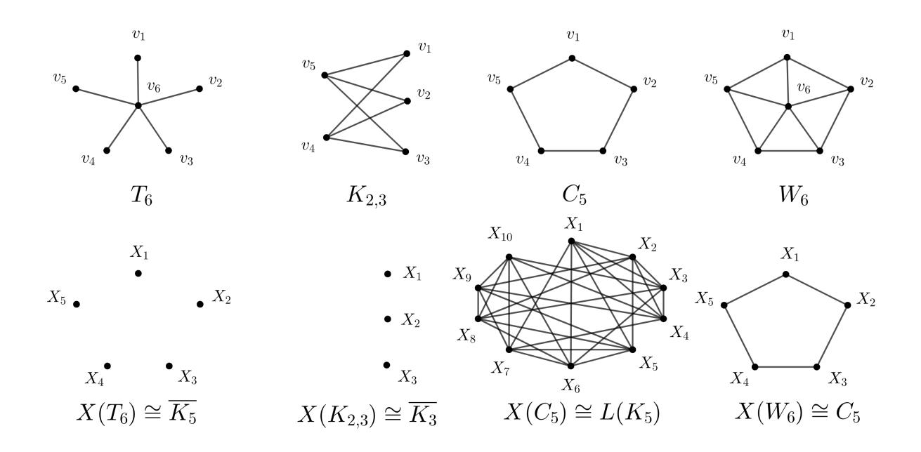
Figure 2. Mincut graphs of some well-known classes of graphs.

Proposition 3.3. Let G be a graph of order n, minimum degree δ and maximum degree ∆. Then G is super-λ if any of the following conditions are satisfied:

• 1. Let G ̸= Kn/² × K2, the cartesian product of Kn/² and K2. If for any non-adjacent u, v ∈ V (G), deg(u) + deg(v) ≥ n, then G is super-λ.
• 2. If for any non-adjacent u, v ∈ V (G), deg(u) + deg(v) ≥ n + 1, then G is super-λ. This is a corollary to the preceding condition.
• 3. If δ ≥ ⌊ⁿ 2 ⌋ + 1, then G is super-λ.
• 4. If G has diameter 2 and contains no complete subgraph H on δ vertices with degGv = δ for all v ∈ V (H), then G is super-λ.
• 5. If G has diameter 2 and n > 2δ + ∆ − 1, then G is super-λ.

Proposition 3.4. If G is super-λ and r-regular, G ≇ K2, then X(G) ∼= G.

Proof. If G is r-regular and super-λ, then V (H) = {v ∈ V (G)|deg(v) = δ(G)} = V (G) and the edge-set incident on every vertex is a mincut. Hence, if viv^j ∈ E(G), then Xⁱ ∩ X^j ̸= ∅ and xix^j ∈ E(X(G)) and isomorphism follows. We exclude K² since K² ∼= T² and X(T2) ∼= K¹ as we saw in Section 2.1.

Definition 3.5. A strongly regular graph is a regular graph G with parameters srg(v, r, λ, µ), where v is the order and r the regularity of G, such that every two adjacent vertices have λ neighbours in common and every two non-adjacent vertices have µ neighbours in common.

The following Lemma is well known in the literature.

Lemma 3.6. The line graph of a complete graph \(L(K_n)\) is a strongly regular graph with parameters \(srg(\binom{n}{2}, 2(n-2), n-2, 4)\).

Corollary 3.7. Let \(K_n\) be the complete graph on n vertices, \(K_{n,n}\) the complete bipartite graph with equal vertex partitions and \(L(K_n)\) the line graph of the complete graph. If n > 2, then

• 1. \(X(K_n) \cong K_n\)
• 2. \(X(K_{n,n}) \cong K_{n,n}\)
• 3. \(X(L(K_n)) \cong L(K_n)\).

Proof. We exclude n=2, since \(K_2\) is a tree, \(K_{2,2}\cong C_4\) and \(L(K_2)\cong K_1\). If n>2 all three graphs are regular and super-\(\lambda\).

For \(K_n\) we have \(\delta = n - 1 \ge \lfloor \frac{n}{2} \rfloor + 1\) for \(n \ge 3\) and hence \(K_n\) is super-\(\lambda\) by condition 3 of Proposition 3.3.

It is fairly straight forward, although lengthy, to show that \(K_{n,n}\) and \(L(K_n)\) are super-\(\lambda\) by condition 4 of Proposition 3.3.

The three graphs are respectively n-1, n and 2(n-2) regular and hence isomorphic to their mincut graphs by Proposition 3.4.

4. When is a Graph a Mincut Graph?

In this section we address the question of which graphs are mincut graphs, that is, which graphs lie in the image of the mincut operator, which we will refer to as the X-operator and denote as \(X(\cdot)\). We show that every graph is a mincut graph, by constructing a super-graph \(G^*\) from a given graph G such that G is the mincut graph of \(G^*\). Furthermore, we show that every graph G has an infinite number of X-roots, that is, graphs that are mapped to G by \(X(\cdot)\). For more on the concepts and definitions on graph operators used here, see Prisner in [16].

Definition 4.1. A graph operator is a mapping \(\phi\) which maps every graph G from some class of graphs to a new graph \(\phi(G)\).

We define the operator recursively, such that, if \(\phi\) is an operator and k a positive integer, then \(\phi^1 = \phi\) and \(\phi^k(G) = \phi(\phi^{k-1}(G))\), for \(k \ge 2\), see [16, 17]. Since an operator, \(\phi\), is a mapping on the set of finite graphs into itself, it is natural to ask which graphs lie in the image of \(\phi\) and, given \(\phi(G)\), are we able to determine G?

Every graph is an intersection graph, see [5, 10]. We show that every graph is the mincut graph of not just one graph, but more. It is possible to construct an infinite family of non-isomorphic graphs that map to the same mincut graph.

Lemma 4.2. Let G be a super-\(\lambda\) graph with \(H \subseteq G\) the induced subgraph on the set of vertices of G such that \(V(H) = \{v \in V(G) | deg(v) = \delta(G)\}\), then \(H \cong X(G)\).

Proof. Let \(x_i \in V(X(G))\) be the vertex in X(G) corresponding to the mincut \(X_i \in X\), the set of all mincuts in G. Since G is super-\(\lambda\), the mincuts of G are exactly the incident edge-sets on the vertices \(v \in V(H)\) and hence |X| = |V(H)|. Thus for every \(v_i \in V(H)\) there is exactly one

\(x_i \in V(X(G))\). Furthermore, if \(v_i v_j \in E(H)\) then \(X_i \cap X_j \neq \emptyset\), where \(X_i\) and \(X_j\) are the incident edge sets on \(v_i\) and \(v_j\). If \(v_i v_j \notin E(H)\) then \(X_i \cap X_j = \emptyset\), since they are the incendent edge-sets on \(v_i\) and \(v_j\). Hence \(x_i x_j \in E(X(G))\) if and only if \(v_i v_j \in E(H)\) and isomorphism follows. \(\square\)

Example 4.3. The graph G in Figure 3 is super-\(\lambda\), by Condition 1 of Proposition 3.3 with vertices of minimum degree \(v_1, v_2, v_3\), and \(v_4\) and \(X(G) \cong K_{1,3}\) is the induced subgraph on vertices \(v_1 \dots v_4\).

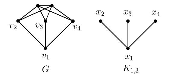
Figure 3. Super-\(\lambda\) graph

Definition 4.4. The join \(G = G_1 \vee G_2\) of two graphs \(G_1\) and \(G_2\) has vertex set \(V(G_1) \cup V(G_2)\) and edge set \(E(G_1) \cup E(G_2) \cup \{uv | u \in V(G_1), v \in V(G_2)\}.\)

In other words, the join of two graphs joins every vertex in the one graph to every vertex in the other graph. Thus, for example, we can say \(K_n = K_1 \vee K_{n-1}\) and \(K_{m,n} = \overline{K_m} \vee \overline{K_n}\). If one of the graphs is \(K_1\) the operation is also called the vertex join of the graph.

Theorem 4.5. Every graph G is the mincut graph of an infinite family of graphs.

Proof. Let G be a graph of order p, not necessarily connected. Let \(K_q\) be a complete graph of order q=p+5 and \(G^*\cong G\cup K_q\), the disjoint union of G and \(K_q\). We note that \(n=|V(G^*)|=2p+5\). Add edges between G and \(K_q\) until \(deg_{G^*}(v)=p+3\) for all \(v\in V(G)\).

Now \(deg_{G^*}(u) + deg_{G^*}(v) = 2p + 6\) for all non-adjacent \(u, v \in V(G)\) and \(deg_{G^*}(u) + deg_{G^*}(x) \ge p + 3 + p + 4 = 2p + 7\) for all \(u \in V(G)\) and \(x \in V(K_q)\). Thus we have \(deg_{G^*}(u) + deg_{G^*}(v) \ge 2p + 6 \ge n + 1\) for all non-adjacent \(u, v \in V(G^*)\) and we conclude that \(G^*\) is super-\(\lambda\) by condition (2) of Proposition 3.3. We also have \(\delta(G^*) = p + 3\) and the vertices of minimum degree in \(G^*\) are exactly the vertices of G. Hence, by Lemma 4.2, \(G \cong X(G^*)\).

If we now join \(K_m\), \(m \geq 1\) and \(G^*\), the order of \(K_m \vee G^*\) is m+2p+5, the degree of each vertex in \(G^*\) increases by m and the degree of each vertex in \(K_m\) is now m+2p+4. For any non-adjacent \(u, v \in V(G)\), \(deg_{K_m \vee G^*}(u) + deg_{K_m \vee G^*}(v) = 2m+2p+6 > m+2p+6\) and for any non-adjacent \(u \in V(G)\) and \(x \in V(K_q)\), \(deg_{K_m \vee G^*}(u) + deg_{K_m \vee G^*}(x) \geq m+p+3+m+p+4 = 2m+2p+7 > m+2p+6\). We have \(\delta(K_m \vee G^*) = p+3+m\), that is the degree of the vertices of the original graph G in \(K_m \vee G^*\). Condition (2) of Proposition 3.3 holds and by Lemma 4.2, \(G \cong X(K_m \vee G^*)\), for any choice of m.

We note that the join of any K^m with just K^q in G^∗ would also give us a super-λ graph with G the induced subgraph on vertices of minimum degree, but then the sufficient condition 2 from Proposition 3.3 would not necessarily hold.

Example 4.6. The graph G in Figure 4 is the mincut graph of a family of super-λ graphs F(G^∗ ) such that G ⊆ G^∗ and V (G) = {v ∈ V (G^∗ )|deg(v) = δ(G^∗ )}. In the first diagram we have G^∗ , the disjoint union of G, of order 4, and K9, of order 4 + 5 = 9. We note that the order of G^∗ is 13. In the second diagram we add edges between G and K⁹ until we have degG^∗ (v) = 7 for all v ∈ V (G). Now degG^∗ (v) ≥ 8 for all v ∈ V (K9) and δ(G^∗ ) = 7. For any two nonadjacent vertices u, v ∈ V (G) we have degG^∗ (u) + degG^∗ (v) = 14 and for any two non-adjacent vertices v ∈ V (G) and x ∈ K⁹ we have degG^∗ (v) + degG^∗ (x) ≥ 15 > 14. Thus, for any two non-adjacent vertices in G^∗ we have that the sum of their degrees is greater than or equal to 14, or n + 1 and we conclude that G^∗ is super-λ. By Lemma 4.2 we have that G is the mincut graph of G^∗ . Furthermore, we could now join any K^m to G^∗ and G would still be the induced subgraph on vertices of minimum degree.

Figure 4. Graphs G and K9, with G^∗ constructed such that X(G^∗ ) ∼= G.

Corollary 4.7. For any connected graph G there is a non-isomorphic graph H such that X(G) ∼= X(H).

5. Roots and Depth

In this section we start to explore some further ideas around the mincut operator. Since we have shown that every graph is a mincut graph we have some immediate consequences for the roots and depth, see [16, 17] of any graph under X(·).

Definition 5.1. For a given graph operator ϕ, a ϕ-root of a graph G is any graph H with ϕ(H) ∼= G.

With respect to roots and iteration we also have the following definition of the depth of a graph under some operator.

Definition 5.2. For a graph G and an operator \(\phi\) we define the \(\phi\)-depth, depth(G), as the largest integer, d, (if there is one, otherwise \(\infty\)) for which there is some graph H such that \(\phi^d(H) \cong G\).

Proposition 5.3. Every graph G has an infinite number of X-roots.

Proof. The proof follows directly from the construction in Theorem 4.5. By our construction \(X(G^*) \cong G\) and it followed that for any choice of \(m, X(K_m \vee G^*) \cong G\).

Proposition 5.4. Every graph G has infinite X-depth.

Proof. By Theorem 4.5, every graph is the mincut graph of a family of graphs. Therefore, given a graph \(G_0\), there is some graph \(G_{(-1)}\) such that \(X(G_{(-1)}) \cong G_0\), where the value of the subscript is merely to indicate position in a sequence. By the same reasoning, there is a graph \(G_{(-2)}\) such that \(X(G_{(-2)}) \cong G_{(-1)}\). Thus we can construct a set \(\{\ldots, G_{(-3)}, G_{(-2)}, G_{(-1)}, G_0\}\) where every \(X(G_{(-n)}) \cong G_{(-n+1)}\) for all \(n \geq 1\) and \(X^n(G_{(-n)}) \cong G_0\).

Example 5.5. We refer to the graphs in Figure 5. Each sequence represents a number of iterations under \(X(\cdot)\). We know that \(X(P_4) \cong \overline{K_3}\) since it is basically a tree on four vertices, and since \(\overline{K_3}\) is disconnected \(X(\overline{K_3}) \cong K_0\) by Lemma 2.4. The graph \(G_1\) was obtained from \(P_4\) by the construction in Theorem 4.5 using \(P_4 \cup K_2\). We note that any graph with exactly three mincuts that do not intersect is also a root of \(\overline{K_3}\) and any disconnected graph is a root of \(K_0\). In the second iteration sequence we have \(C_4\) as a root of \(L(K_4)\). We could have constructed a root using our construction method from Theorem 4.5 or, since line graphs of complete graphs are fixed under \(X(\cdot)\) we could simply have \(L(K_4)\). \(W_5\) is a root of \(C_4\) since \(W_5 \cong K_1 \vee C_4\) and \(C_4\) is 2-regular with n=4>2+1. We could apply our construction technique again to \(G_1\) and \(W_5\) respectively to continue each sequence in reverse and generate an infinite sequence of graphs such that each is an X-root of the next. Admittedly our graphs will become very large very soon but it is possible in principle.

Figure 5. Graphs with some of their X-roots.

6. Further Discussion

In this section we conclude by introducing and exploring further topics and questions raised by the properties and characteristics of the mincut graph.

We also look at the possible implications of certain induced subgraphs in X(G) for a root if that root is not necessarily obtained from the construction process in Theorem 4.5.

6.1. Determination Problem

We know from Whitney that a graph is uniquely determined by its line graph up to isolated vertices, unless it is \(C_3\) or \(K_{1,3}\), see [17]. Although our construction in Theorem 4.5 gives the interesting result that every graph is a mincut graph, it unfortunately does not shed much light on what the mincut graph X(G) tells us about the mincuts of G if G is not a graph of the family obtained by our construction. We explore this problem in a little more detail.

Lemma 6.1. Let \(X = \langle A, \overline{A} \rangle\) and \(Y = \langle B, \overline{B} \rangle\) be two non-trivial mincuts of a graph G with \(A, \overline{A}\) and \(B, \overline{B}\) the vertex sets of the components of G - X and G - Y respectively. If \(X \cap Y \neq \emptyset\) then either \(A \cap B \neq \emptyset\) or \(A \cap \overline{B} \neq \emptyset\).

We note that the converse to Lemma 6.1 is not necessarily true.

We know, see [2, 12], that if \(X = \langle A, \overline{A} \rangle\) and \(Y = \langle B, \overline{B} \rangle\) are two mincuts of G and \(A \cap B \neq \emptyset\) then either \(A \subset B\) (or \(B \subset A\)), that is they are nested, or they overlap. If X and Y overlap (also called crossing mincuts), then \(A \cap B\), \(\overline{A} \cap B\) and \(A \cap \overline{B}\) are non-empty. We also note from [12] that two mincuts can overlap only if \(\lambda\), the minimum edge connectivity number of the graph, is even.

Proposition 6.2 (Lehel et al, [12]). Let \(X = \langle A, \bar{A} \rangle\) and \(Y = \langle B, \bar{B} \rangle\) be two overlapping mincuts of a connected graph G. Then \(|\langle \bar{A} \cap \bar{B}, A \cap \bar{B} \rangle| = |\langle \bar{A} \cap \bar{B}, \bar{A} \cap B \rangle| = |\langle A \cap B, A \cap \bar{B} \rangle| = |\langle A \cap B, \bar{A} \cap B \rangle| = \frac{\lambda}{2}\). Consequently \(A \cup B\), \(A \cap B\), \(A \cap B\), \(\bar{A} \cap B\) are mincuts. Moreover, \(|\langle \bar{A} \cap \bar{B}, A \cap B \rangle| = |\langle \bar{A} \cap B, A \cap \bar{B} \rangle| = 0\).

Lemma 6.3 (Chandran & Ram, [2]). If \(X = \langle A, \overline{A} \rangle\) and \(Y = \langle B, \overline{B} \rangle\) are a pair of crossing mincuts, then \(X \cap Y = \emptyset\).

Let \(X=\langle A,\bar{A}\rangle\) and \(Y=\langle B,\bar{B}\rangle\) be overlapping mincuts of a graph G with non-trivial mincuts \(W=\langle A\cap B,\bar{A}\cup\bar{B}\rangle, Z=\langle A\cup B,\bar{A}\cap\bar{B}\rangle\) as per Proposition 6.2. Suppose that \(W\cap X,Y\) and \(X,Y\cap Z\) are non-empty, then we have a corresponding induced cycle \(C_4\) in X(G). Given what we know from Proposition 6.2, it would seem that we should at least be able to construct an induced subgraph in G corresponding to the cycle in X(G) without resorting to the construction in Theorem 4.5.

Similarly, let \(X = \langle A, \bar{A} \rangle\), \(Y = \langle B, \bar{B} \rangle\) and \(Z = \langle C, \bar{C} \rangle\) be non-trivial nested mincuts of a graph G with \(A \subset B \subset C\). If the induced subgraph in X(G) corresponding to the mincuts X, Y and Z is connected then we should have a cycle \(C_3\) or at least an induced path \(P_3\) in X(G).

It would be interesting to know whether we can have induced cycles larger than \(C_4\) in X(G) such that the corresponding mincuts in G are not of the form as per our construction in Theorem 4.5.

6.2. Periodicity of the Mincut Operator

Definition 6.4. Let \(\phi\) be an operator on a class of graphs \(\Gamma\). A graph \(G \in \Gamma\) is periodic in \(\phi\) if there is some natural number n with \(G \cong \phi^n(G)\). The smallest such number is called the period of G.

In Corollary 3.4 we showed that it is sufficient for \(G \cong X(G)\) if G is super-\(\lambda\) and r-regular. That is, the graph is fixed under the operator, or has periodicity 1. In fact, it can be shown that this condition is also necessary.

Furthermore, we know that there are 2-periodic graphs under \(X(\cdot)\). For example, the cartesian product \(K_m \times K_2\) has mincut graph \(X(K_m \times K_2) \cong K_1 \vee (K_m \times K_2)\), the join of itself with \(K_1\). But the mincut graph of \(K_1 \vee (K_m \times K_2)\) is again \(K_m \times K_2\) which means that iteration of the \(X(\cdot)\) operator leads to a cycle of two graphs. A natural question to ask is whether there are other graphs of this periodicity and if so what would be their characteristics. Furthermore, do we have graphs of a higher X-periodicity?

6.3. Convergence or Divergence

In [18] Wilf and Van Rooij showed that unless a graph is \(K_{1,3}\), \(C_n\) or \(P_n\), repeated application of the line graph operator eventually leads to a steadily increasing number of vertices, that is, it diverges under \(L(\cdot)\).

We know that the maximum number of mincuts in a graph of order n is \(\binom{n}{2}\) and this bound is tight for simple graphs when \(G \cong C_n\), see [4, 12]. We also have other upper bounds on the number of mincuts of a graph depending on whether \(\lambda\) is even or odd as mentioned in Section 1.

Intuitively, if a graph is to diverge under \(X(\cdot)\) both the number of vertices and edges need to increase. If only the number of vertices increases the edge density of the graph decreases and the likelihood of every mincut intersecting with at least one other decreases, converging to the null graph in the end. If only the number of edges increases we eventually end up with a complete graph which is fixed. But for |V(X(G))| and |E(X(G))| to increase and X(G) to remain connected we must have the edge density increasing. Thus we would expect such a graph to eventually become fixed (or at least periodic) under the X-operator.

Hence, given the upper bounds on the number of mincuts, that we expect graphs that "grow" to eventually become fixed or periodic, that non-intersecting mincuts are disconnected and that the mincut graph of a disconnected graph is the null graph, \(K_0\), we have the following two conjectures:

Conjecture 1 (Convergence). Let G be a simple connected graph and \(X(\cdot)\) the mincut operator. Then \(X^n(G)\) converges for sufficiently large n.

Conjecture 2 (Convergence to null graph). Let G be a simple connected graph and \(X(\cdot)\) the mincut operator. Then \(X^k(G) \to K_0\) for sufficiently large k, except under a finite number of conditions.

6.4. Connectivity of X(G)

X(G) will be connected if every mincut has non-empty intersection with at least one other mincut. What are the characteristics of a connected graph that will imply that its mincut graph is connected? Is it possible to find minimum bounds on κ(G), λ(G), and δ(G), (the vertex connectivity, edge connectivity and minimum degree values of G) that will guarantee a connected X(G)? Intuitively there should be some relationship between the vertices and the way the edges are distributed (some kind of "edge density" function?) and λ(G) that will ensure connectivity of X(G).

Acknowledgement

The authors would like to thank the reviewers for their valuable comments in strengthening this paper.

References

• [1] L. Cai, D. Corneil, and A. Proskurowski, A generalization of line graphs: (X,Y)-intersection graphs, J. Graph Theory 21 (3) (1996), 267–287.
• [2] L.S. Chandran and L.S. Ram, On the Number of Minimum Cuts in a Graph, SIAM J. Discrete Math. 18 (1) (2004), 177–194.
• [3] D. Chartrand, L. Lesniak, and P. Zhang, Graphs and Digraphs, 5th ed., CRC Press, Boca Raton, 2011.
• [4] E. Dinic, A. Karzanov, and M. Lomosonov, The structure of a system of minimal edge cuts of a graph. In A.A. Fridman, editor, Studies in Discrete Optimization, pages 290–306. Nauka, Moscow, 1976. Note: Translation at http://alexander-karzanov.net/ ScannedOld/76_cactus_transl.pdf.
• [5] P. Erdos, A.W. Goodman, and L. Posa, The representation of a graph by set intersections, Can. J. Math. 18 (1966), 106–112.
• [6] L. Fleischer, Building Chain and Cactus Representations of All Minimum Cuts from Hao-Orlin in the Same Asymptotic Run Time, Journal of Algorithms 33 (1999), 51–72.
• [7] H.N. Gabow, A Matroid Approach to Finding Edge Connectivity and Packing Arborescences, Journal of Computer and System Sciences 50 (2) (1995), 259–273.
• [8] M.C. Golumbic, Algorithmic Graph Theory and Perfect Graphs, 2nd ed., Elsevier, Amsterdam, 2004.
• [9] J.L. Gross, and J. Yellen, Handbook of Graph Theory, 1st ed., CRC Press, Boca Raton, 2004.
• [10] F. Harary, Graph Theory, Addison-Wesley, Reading, 1969.

• [11] A. Kanevsky, Graphs with odd and even edge connectivity are inherently different, Tech. report, TAMU-89-10, 1989.
• [12] J. Lehel, F. Maffray, and M. Preissmann, Graphs with largest number of minimum cuts, Discrete Appl. Math. 65 (1996), 387–407.
• [13] L. Lesniak, Results on the edge-connectivity of graphs, Discrete Math. 8 (1974), 351–354.
• [14] T.A. McKee and F.R. McMorris, Topics in Intersection Graph Theory, SIAM, Philadelphia, 1999.
• [15] M. Pal, Intersection Graphs: An Introduction, Annals of Pure and Applied Mathematics, 4 (1) (2013), 43–91.
• [16] E. Prisner, Graph Dynamics, Longman, Harlow, 1995.
• [17] E. Prisner, Line Graphs and Generalizations – A Survey. In G. Chartrand and M. Jacobson, editors, Surveys in Graph Theory, pages 193–229. Util. Math., Winnipeg, 1996.
• [18] A.C.M Van Rooi and H.S. Wilf, The interchange graph of a finite graph, Acta Math. Hungar. 16 (3–4) (1965), 263–269.