Ridi Ferdiana1 , Wiliam Fajar Dicka2 and Alfred Boediman3
1.2Department of Electrical and Information Engineering, Universitas Gadjah Mada, Yogyakarta, Indonesia 3Samsung Research Indonesia, Jakarta, Indonesia ridi@ugm.ac.id, wiliam.fajar.d@mail.ugm.ac.id, alfred.b@samsung.com
Abstract: In this study, we attempt to use a convolutional neural network (CNN) to identify cats' different sounds. CNN is proven to classify different patterns from the spectro-temporal features of a sound and thus well suited for sound classification. We will perform data transformation using mel-frequency cepstral coefficients (MFCCs) to extract the sound frequency to apply this method. In MFCCs, each frequency bin is quasi-logarithmically spaced so that it resembles the resolution of the human auditory system compared to the spectrogram. We will be using four convolutional layers of CNN architecture with a pooling layer and dense layer as the output layer in our model. From the sound ontology Audio set, we can collect 595 different sound data classified into five categories of cat sounds, which we used to train our model. From our training process, our model can achieve a classification accuracy of 88.473254%. In the future, we look forward to improving our model accuracy by adding more data and even out each label to reduce overfitting. We would also like to implement a data augmentation method on our dataset to improve our model accuracy.
Keywords: Convolutional Neural Network (CNN), deep learning, Mel-frequency cepstral coefficients (MFCCs), sound classification
1. Introduction
An artificial neural network or just a neural network is a machine learning algorithm that consisted of nodes and neurons which pass information to one another. It offers flexibility in its application allowing a neural network to be used in various problems in real life [1]. This comprehensive application also pushes different network architecture models based on the neural network [2]. One of the most famous architectures of an artificial neural network is the convolutional neural network (CNN).
A convolutional neural network is most commonly used and widely acknowledged for performing pattern and visual recognition for various image classification tasks [3-4]. Convolutional neural networks in the field of image classification can be applied to a wide range of problems from classifying traffic signs [5] to handwriting [6] and even able to detect brain tumors [7]. Right now, the application of a convolutional neural network is also used in the field of sound classification. The most common application of a convolutional neural network is sound classification is to classify general or environmental sounds [8-10]. A convolutional neural network can be applied for sound classification by transforming the sound data as spectrogramlike inputs and then identifying the patterns on said inputs [11-12]. This way, the model can distinguish different noise-trait from different sources of sounds.
Animal sound classification with CNN while has been gaining traction, is still only a fraction of total study in the field on sound classification. Furthermore, animal classification outcome is often more focused to determine species of the animal rather than the emotion based on their sound [19-20]. With this paper we try to shift our focus from species classification to emotion classification based on animal sound, specifically cats.
The problems with sound classification are the difficulty of acquiring a huge amount of data that is consistent. Consistency in sound data is harder to achieve compared to image data. Sound data is more prone to noises and more affected by different capturing devices and compression. Some audio feature visualization methods such as Mel-frequency cepstrum can help in mitigating noise in sound data [13]. The convolutional neural network also needs large quantities
Received: January 5th, 2021. Accepted: September 29th, 2021
DOI: 10.15676/ijeei.2021.13.3.15
and balanced data to avoid overfitting, which is where the data will perform well on training data but poorly on real data.
In this paper, we applied a convolutional neural network to perform a sound classification of different noises made by cats. Our data consists of cat sounds that are labeled as emotions. Our model will then be used to classify these emotions based on cat sounds. To do that, we perform feature extraction with Mel-frequency cepstral coefficients (MFCCs), which are collective coefficients of Mel-frequency cepstrum. We will discuss the architecture of the CNN with the feature generated by MFCCs and its score performance.
Different noises of cats often linked to distinctive behaviour or emotions, with this paper as a foundation we planned to build an algorithm to detect cats emotion not only based on noise, but also on implement species, gender, and age to more accurately interpret cat's emotion based on its sound. Sadly, there are not enough data about cat sound classification that incorporate above characteristic, therefore we also plan to built a mobile application to provide services of detecting cat's emotion based on sound and those characteristic while also using those data and feedback to build the algorithm.
2. Method
A. Convolutional Neural Network
Convolutional Neural Network is a class of deep neural network built based on a multilayer perceptron model. This convolutional layer each consisted of multiple neurons or nodes that are interconnected to the next layer [14] and stacked together to construct a deep architecture. CNN is built upon Each point of data and then will be fitted to these layers so that our model can learn high-level hierarchical feature from our data [15].
Figure 1. Convolutional neural network model used in this study.
In this study, our model will be built with four convolutional layers, with the output layer as a dense layer. A dense layer means that all the nodes from the previous layer will be fully connected. For out input layer, the input layer will receive the input shape of (40, 431, 1). This input shape is based on the Mel-frequency cepstral coefficients (MFCCs) transformation of our data. The data we will be using will be transformed into 40 coefficients. We will be taking the maximum number of frames from each number of coefficients. For our data, the number of frames on each MFCCs is approximately 431. Therefore we will apply zero paddings on the output of transformation to equalize the number of frames. So, our layer will be 2-dimensional layers.
The convolutional kernel will inspect our data in the specified dimension until the entire data is analyzed. The dot product of the operation will then be calculated and passed to the next layer. The small size of the layer compared to our input size will allow our model to learn the pattern in a more localized way and more thorough in detecting the presence of specific elements in sound classes even with the existence of noises.
For each layer, we will also add a pooling layer to reduce our layer's dimensionality and thus can focus on more important parts [16]. On each layer, we also apply a 0.2 dropout to reduce the number of nodes randomly to avoid overfitting. By reducing the number of nodes in each layer, we
will prevent our model from accidentally become too limited to the training data. Implementation of dropout makes so that our nodes did not become too dependent on other nodes and make the nodes learning process priorities the feature itself.
On this experiment, we will use 4-layer convolutional network architecture. On the input layer, we will start with 16 nodes and then increase it incrementally to 32, 64, and finally, on the final layer, 128 nodes. These layer will be formed with Conv2D algorithm to match our 2-dimensional input shape. For all of the layers, we will use 2 x 2 convolutional window or kernel size, which is the dimension where our model with inspecting the data. On the output layer, we will apply a dense layer so that it is interconnected with the previous layer. Finally, this model will use rectified linear units (relu) as an activation unit. Relu has been shown to bring improvement in learning speed to a deep neural network and thus is used as a standard activation function for the deep neural network [17]. Relu brings computational simplicity, representational sparsity, and linear behavior to the neural network model. Relu activation function simply works by returning the value that is inputted or zero if the input is less than zero.
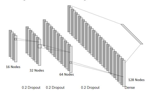
Figure 2. Simplified convolutional diagram used in this experiment.
B. Mel-frequency Cepstrum
Mel-frequency cepstrum (MFC) is a visual representation of sounds as a spectrum, like a spectrogram. Mel-frequency cepstral coefficients (MFCCs) are coefficients that make up an MFC. In MFCCs, each frequency bin is quasi-logarithmically spaced roughly, resembling the resolution of the human auditory system compared to the standard spectrogram, which has an equal number of hertz for each frequency bin space. This makes MFCCs have a more biologically inspired feature and perform better in speech recognition and segregation [18] as well as in animal sound classification [19]. Another example of time-frequency representations (TFRs) that can be used for animal sound classification is harmonic-component based spectrogram and percussive-component based spectrogram [20].
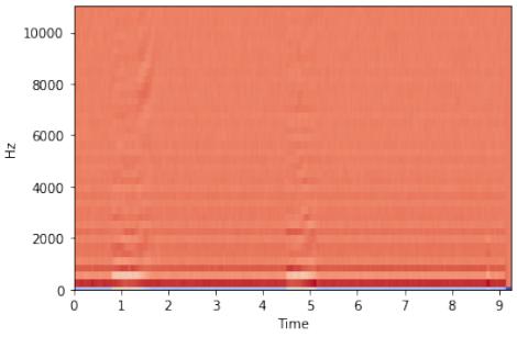
Figure 3. Visualizing cat's meowing sound using MFCCs
We used librosa to calculate the MFCCs values of our data. Librosa calculate MFCCs values by using Discrete Cosine Transform (DCT) on mel-scaled spectrogram of our data that is converted
into decibel. We use the type II of DCT and then take the first 40 coefficient as MFCCs. The formula for calculating DCT type II is \(X_k = \sum_{n=0}^{n-1} x_n \cos\left[\frac{\pi}{N}\left(n+\frac{1}{2}\right)k\right]\) where x the mel-scaled spectrogram value which converted to decibel unit.
MFCCs can visualize our data in the shape of a heat map-like figure. This figure can be quantized based on the number of coefficients specified and the sample rate of the audio. The result of an MFCCs visualization can be seen in Figure 2.
C. Dataset
We will collect the data from a human-labeled audio ontology called an audio set. Each entry of an audio set is a 10-second sound clip that is drawn from YouTube videos. From this ontology, we will take sound data that is categorized as cat sound data. These data categorization consists of purring, which is a sound made by cats to indicate relaxed pleasure, meowing which is a classic tonal communication made by cats, hissing which is a sound when a cat is giving a warning or indicating disapproval, caterwaul, which is the yowling sound made by a cat in heat, and growling which is a sign of aggression or expression of anger from cats.
D. Other Studies
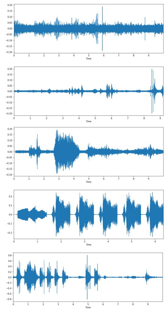
Figure 4. Oscillogram of each of the cat sound samples, from top to bottom: purr, meow, growling, hiss, caterwaul.
There have been some studies conducted about sound classification on animals which specifically using convolutional neural network or its variations. For example, E. Şaşmaz and F. B. Tek in "Animal Sound Classification Using A Convolutional Neural Network" conduct a research to identify 10 different animals based on sound using convolutional neural network with different optimizers [19]. In said study, E. Şaşmaz and F. B. Tek is able to achieve the best accuracy of 75% using NADAM (Nesterov-accelerated Adaptive Moment Estimation) as the optimizers.
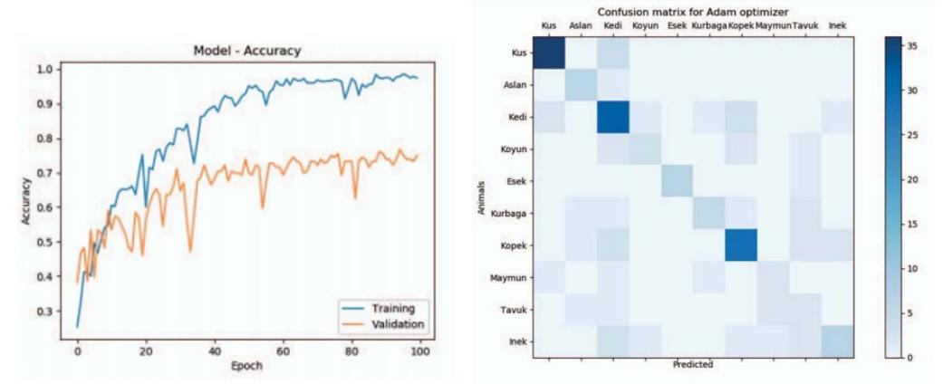
Figure 5. Accuracy and Confusion matrix from "Animal Sound Classification Using A Convolutional Neural Network".
In "Investigation of Different CNN-Based Models for Improved Bird Sound Classification", J. Xie, K. Hu, M. Zhu, J. Yu and Q. Zhu combine three CNN model with different TFRs (Time-Frequency Representation) in a VFF style network [20]. With this model they were able to achieve a balanced accuracy of 86.32% and weighted F1-score of 93.31%
3. Experiment and Results
A. Data Collection
In this study, we will be using a sound dataset from an audio set. We will be choosing data based on a specific label on the audio set. The label that we choose is purr, meow, growling, hiss, and caterwaul. Each of these sounds will be used to interpret a specific sound of cats. Purring is categorized as happy or relaxed, meowing is categorized as neutral, growling is categorized as anger or aggression, hissing is categorized as cautious or tense, and caterwaul is categorized as lonely. The visualization of each sound can be seen in Fig. 3.
Audio set on cat sounds consists of 3,964 data. But, due to the nature of the ontology itself, data on the audio set can consist of multiple labels. We choose to collect data that only have our specified label (purr, meow, growling, hiss, and caterwaul) and nothing else. Some of the data from the audio set are also unavailable because the video on youtube is deleted or is not available in Indonesia. In the end, we managed to collect 595 data divided into five labels that can be seen in Table 1.
| Label | Quantity |
|---|---|
| Purr | 168 |
| Meow | 107 |
| Growling | 70 |
| Hiss | 146 |
| Caterwaul | 104 |
759
The limited number of data will no doubt affect the performance of our model. Even more, the unbalanced amount of data on each label will also affect the performance in negative ways. Despite the limitation of our data, we hope that our model will still perform adequately. In the future, we hoped to perform this experiment with an additional amount and more balanced data.
Each of the data in audio set is linked to a specific youtube video containing the sound and timestamped in a 10-second duration. Thus, in the data collection process, we will download the sound data directly from youtube. For the download process itself, we will be using open-source software called FFmpeg and a python script. We will download the audio portions of the youtube video on the specified timestamps with a 44100 sample rate, two channels, 16-bit depth, and .flac format.
B. Data Transformation
Before we can use our audio data to perform model training, first, we perform a transformation process on our data. In this step, we choose Mel-frequency cepstral coefficients (MFCCs). By using MFCCs, our model will be able to analyze sound frequency on our data in a time-based characteristic. This is because MFCCs summarises frequency distribution on the duration of the data. Fig. 5 is the visualization of MFCCs if compared to a spectrogram.
In this process, we will extract numeric values from the MFCCs. For the MFCCs extraction, we will be taking 40 coefficients from our audio data. We will also specify 431 as the maximum number of features that can be extracted from our data. Thus, after the transformation, the shape of our data is a 40 by 431 two-dimensional matrix.
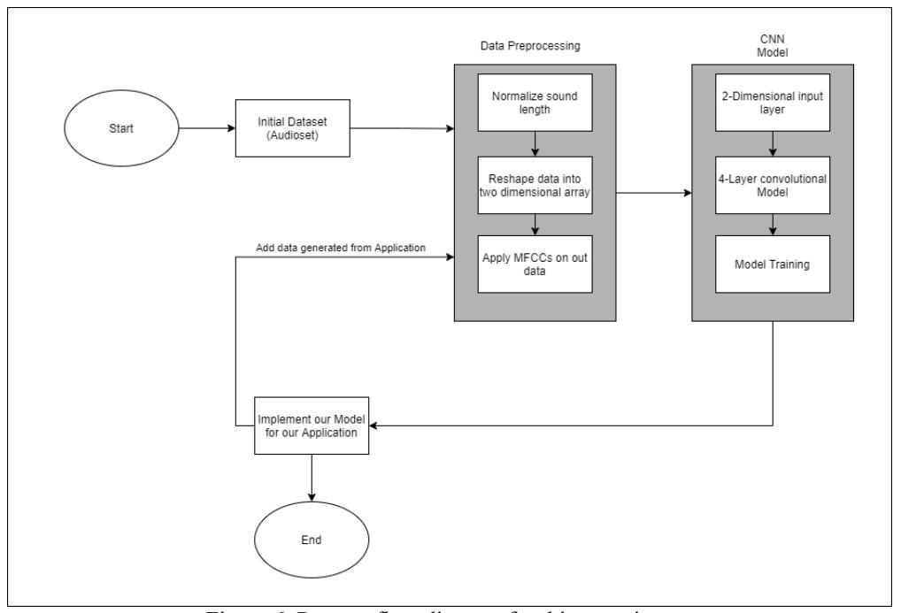
Figure 6. Process flow diagram for this experiment.
C. Experiment
For this study, we choose to use a convolutional model with four layers. Convolutional layers can detect features from data by hovering over the data on specified window size. The bigger the window size, the faster a model can perform training from data, but it also reduces the number of features that can be extracted from data. To balances the speed and the number of features, it is
important to choose the right number of windows on a CNN model. For our model, we decided to use a simple 2x2 windows to perform feature extraction on our 40 by 431 data.
The convolutional neural network consisted of nodes. These nodes are part of our model that performs training and prediction based on the data. For our model, each convolutional layer will have an increasing number of nodes. We will use 16 nodes in the input layer up to 128 nodes on the final layer. Convolutional layers are called convolutional because they work in the same concepts of convolutional filters that are used in image or signal processing. But there is also a dense layer that is used in our output layer. In the dense layer, all the nodes from the previous layer will be connected to the current node, and so for the output layer, there will be five nodes for each type of label that is interconnected to each node from the previous layer.
In our model, we will also apply a pooling layer. This pooling layer will be associated with each of the convolutional layers to reduce the dimensionality of our model. by reducing the dimensionality. We will also reduce the time needed for training. The pooling layer can also reduce overfitting because the dimensionality reduction means our model will less likely develop a dependency on the previous layer.
In the training process, the data will be split into training and testing data. For the training data, we will be using 80% of the dataset, and for the testing data, we will be using 20% of the dataset. For the validation process, we will be using accuracy to measure the performance of our machine learning model.
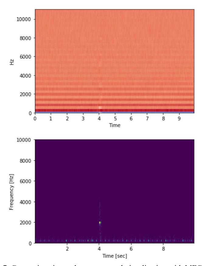
Figure 7. Comparison image between sound visualization with MFCCs (top) and spectrogram (bottom)
4. Result
Because our data has a balanced number of each classification label, and we have 5 different classification label, we use simple accuracy measurement instead of precision, recall, or F1 score. In machine learning, accuracy is simply measured with \(Accuracy = \frac{Correct\ Prediction}{All\ Prediction}\). In our experiment, we calculate the accuracy using keras method model.evaluate. This method also take into account the loss value of our model during the fitting phase into our accuracy.
Our model yields prediction results as follows, on the training data, our model able to predict the sound of a cat correctly 88.473254% percent of the time, but on our testing data, the model only able to predict 70.80734% percent of the time. This means there is approximately a 20% difference between our model performance on training data and testing data.
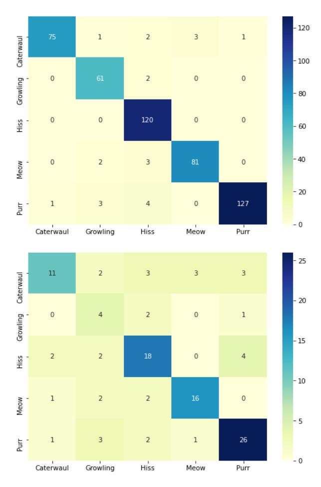
Figure 8. Confusion matrix of the accuracy of our model when classifying training data (top) and testing data (bottom).
This difference between training accuracy and testing accuracy can happen because of overfitting, which is when our model is too accustomed to the training data. We conclude that this happens because our dataset has too few data, and our model cannot perform the training process effectively. The imbalance in our dataset may also affect the testing accuracy of our model, which can be seen on the confusion matrix of the testing data, the growling category, which has the least data in our dataset achieve the least accuracy compared to other category.
To improve our model accuracy when dealing with new data, we will need to increase the number of data is used for training and balanced the data, so each label has the same amount of data, and applying a data augmentation method on our data.
We also show the confusion matrix result of our model to visualize how accurate our model predict each classification label. On the X-axis of the confusion matrix is the predicted value, and on the Y-Axis of the confusion matrix is the actual value. For example on Caterwaul label, we have 75 data correctly predicted, 1 data wrongly predicted as Growling, 2 data wrongly predicted as Hissing, and so on.
5. Conclusion
In this study, we attempt to build a convolutional neural network model that is able to perform sound classification from different kinds of cat sound.
Our model is able to perform well by implementing Mel-frequency cepstrum coefficients transformation on the sound data. From our training process, our model is able to yields relatively high accuracy when compared to another study with different methods, when taking into account the limited number of data available and limited time for the training process. This concludes that the convolutional neural network is indeed effective when used to perform sound classification. The problem that we found in this study is that in our model, due to the limited number of data and the unbalanced state of the dataset, our model is slightly overfitting to the training data.
In the future, we would like to improve our model by expanding our dataset and even out each different category, as well as applying sound augmentation to reduce overfitting and improve our model accuracy.
6. Acknowledgment
-
7. References
- [1]. Nezzar, Reda & Farah, Nadir & Khadir, Mohamed & Chouireb, Lakhdar. (2016). Mid-Long Term Load Forecasting using Multi-Model Artificial Neural Networks. International Journal on Electrical Engineering and Informatics. 8. 389-401. 10.15676/ijeei.2016.8.2.11.
- [2] Tawfeeq, Mohammed. (2020). Optimization of Neural Networks Based on Modified Multi-Sonar Bat Units Algorithm. International Journal on Electrical Engineering and Informatics. 12. 105. 10.15676/ijeei.2020.12.1.9.
- [3]. Krizhevsky, Alex & Sutskever, Ilya & Hinton, Geoffrey. (2012). ImageNet Classification with Deep Convolutional Neural Networks. Neural Information Processing Systems. 25. 10.1145/3065386
- [4]. Russakovsky, Olga & Deng, Jia & Su, Hao & Krause, Jonathan & Satheesh, Sanjeev & Ma, Sean & Huang, Zhiheng & Karpathy, Andrej & Khosla, Aditya & Bernstein, Michael & Berg, Alexander & Fei-Fei, Li. (2014). ImageNet Large Scale Visual Recognition Challenge. International Journal of Computer Vision. 115. 10.1007/s11263-015-0816-y.
- [5]. Cireşan, Dan & Meier, Ueli & Masci, Jonathan & Schmidhuber, Jürgen. (2012). Multi-Column Deep Neural Network for Traffic Sign Classification. Neural networks: the official journal of the International Neural Network Society. 32. 333-8. 10.1016/j.neunet.2012.02.023.
- [6]. Ebrahinpour, Reza & Amini, Mona & Sharifizadehi, Fatemeh. (2011). Farsi Handwritten Recognition Using Combining Neural Networks Based on Stacked Generalization. International Journal on Electrical Engineering and Informatics. 3. 146-164. 10.15676/ijeei.2011.3.2.2.
- [7]. Mohsen, Heba & El-Dahshan, El-Sayed & El-Horbarty, El-Sayed & M. Salem, Abdel-Badeeh. (2017). Classification using Deep Learning Neural Networks for Brain Tumors. Future Computing and Informatics Journal. 3. 10.1016/j.fcij.2017.12.001.
- [8]. Piczak, Karol. (2015). Environmental sound classification with convolutional neural networks. 1-6. 10.1109/MLSP.2015.7324337.
- [9]. Salamon, Justin & Bello, Juan. (2017). Deep Convolutional Neural Networks and Data Augmentation for Environmental Sound Classification. IEEE Signal Processing Letters. PP. 10.1109/LSP.2017.2657381.
- [10]. Abdoli, Sajjad & Cardinal, Patrick & Koerich, Alessandro. (2019). End-to-End Environmental Sound Classification using a 1D Convolutional Neural Network. Expert Systems with Applications. 136. 10.1016/j.eswa.2019.06.040.
- [11]. Salamon, Justin & Bello, Juan. (2015). Feature Learning with Deep Scattering for Urban Sound Analysis. Proceeding 2015 European Signal Processing Conference (EUSIPCO). 10.1109/EUSIPCO.2015.7362478.
- [12]. F. Demir, D. A. Abdullah and A. Sengur, "A New Deep CNN Model for Environmental Sound Classification," in IEEE Access, vol. 8, pp. 66529-66537, 2020, doi: 10.1109/ACCESS.2020.2984903.
- [13]. Cotton, Courtenay & Ellis, Daniel. (2011). Spectral vs. spectro-temporal features for acoustic event detection. IEEE Workshop on Applications of Signal Processing to Audio and Acoustics. 69-72. 10.1109/ASPAA.2011.6082331.
- [14]. Abdel-Hamid, Ossama & Deng, li & Yu, Dong. (2013). Exploring Convolutional Neural Network Structures and Optimization Techniques for Speech Recognition.
- [15]. Sapijaszko, Genevieve & Mikhael, Wasfy. (2018). An Overview of Recent Convolutional Neural Network Algorithms for Image Recognition. 743-746. 10.1109/MWSCAS.2018.8623911.
- [16]. F. Demir, A. M. Ismael and A. Sengur, "Classification of Lung Sounds with CNN Model Using Parallel Pooling Structure," in IEEE Access, vol. 8, pp. 105376-105383, 2020, doi: 10.1109/ACCESS.2020.3000111.
- [17]. Ide, Hidenori & Kurita, Takio. (2017). Improvement of learning for CNN with ReLU activation by sparse regularization. 2684-2691. 10.1109/IJCNN.2017.7966185.
- [18]. Zheng, Fang & Zhang, Guoliang & Song, Zhanjiang. (2001). Comparison of Different Implementations of MFCC. J. Comput. Sci. Technol. 16. 582-589. 10.1007/BF02943243.
- [19]. E. Şaşmaz and F. B. Tek, "Animal Sound Classification Using A Convolutional Neural Network," 2018 3rd International Conference on Computer Science and Engineering (UBMK), Sarajevo, 2018, pp. 625-629, doi: 10.1109/UBMK.2018.8566449.
- [20]. J. Xie, K. Hu, M. Zhu, J. Yu and Q. Zhu, "Investigation of Different CNN-Based Models for Improved Bird Sound Classification," in IEEE Access, vol. 7, pp. 175353-175361, 2019, doi: 10.1109/ACCESS.2019.2957572.
Ridi Ferdiana is a software engineer, lecturer, and Microsoft Certified Trainer who loves to teach and to share with the community. Ridi also an associate professor at Universitas Gadjah Mada. He obtained his doctorate in electrical engineering at the age of 26. His dissertation entitled "An extreme programming approach for global software development" was indexed at ACM SIGSOFT in 2011. Nowadays, Ridi manages the Cloud Experience research group that aligned with his postdoctoral research that focused on modern enterprise and software engineering methodology; technology-enhanced
learning and optimization; cloud adoption & cognitive application. Ridi is also a Microsoft Most Valuable professional in DevOps for more than 13 years with 16 international certifications for Microsoft. In his spare time, Ridi enjoying his spare time as Xbox Ambassador, Car detailer, auto geeks, and eSport player for driving simulation.
Wiliam Fajar is a software engineer and researcher at MIC Enterprise. Wiliam completed his bachelor's degree in 2019 at Universitas Gadjah Mada. On Academia field, Wiliam focuses his research and publishing paper on Data and Machine Learning while on Professional field he is specialized on Microsoft .NET Framework. Wiliam spend his free time playing badminton hand video games.
Alfred Boediman is an experienced senior management who has implemented changes to answer business and technology needs across some areas in the technology and finance sectors. Alfred also an Adjunct Professor at the University of Chicago, Graduate School of Business-Asia Campus; he holds degrees from Universitas Indonesia, Vrije Universiteit Brussel, Rochester Institute of Technology, and the University of Chicago. His postdoctoral research examines the neuro-statistical approach in derivatives financial
exchange combined with multi-layered market sentiment. Alfred's interested and trained in technology research for cognitive socio-behaviour and machine learning area. He is also an angel investor for several tech startups and advisor for Polsky Center for Entrepreneurship at the University of Chicago (Asia chapter); while enjoying organizational activities like Vespa riding, biking, archery, and cooking in his free time.