
Introduction
In the fast development of infrastructure, the presence of strong and safe bridges is important in facilitating efficient mobility of both individuals and commodities. Nevertheless, as the demands imposed on bridges escalate over time, the potential for a decrease in their load-bearing capacity is evident. Consequently, there is an imperative need for periodic assessment of existing bridges to detect structural damage or vulnerabilities arising from factors such as aging, fatigue, or environmental influences. Such assessments are crucial in ascertaining whether a bridge conforms to the applicable safety and capacity standards. The seismic evaluation of bridges has heightened importance especially in regions like Indonesia, which is situated within the seismic Ring of Fire. Despite this, the Indonesian context is characterized by the absence of official regulations delineating procedures for scrutinizing the capacity and seismic performance of bridge structures. This lacuna underscores the urgency for more concerted efforts aimed at enhancing the safety and reliability of bridges in Indonesia. Confronting this challenge requires the adoption of a rigorously tested and dependable methodology for the assessment of bridge capacity and seismic performance.
In this particular framework, AASHTO's The Manual for Bridge Evaluation [1] outlines methodologies for assessing the capacity of bridge structural elements under live loads. The Load & Resistance Factor Rating (LRFR) presented in the document integrates load factors and safety factors to enhance the precision and conservatism of bridge structure capacity evaluations. Comparative studies by Toutanji et al. [2] and Estes et al. [3] demonstrated that LRFR yields more conservative values for various parameters. This method finds applicability in conjunction with the SHMS system, as evidenced by its utilization in the research conducted by Al-Khateeb et
al. [4]. Additionally, the NCHRP Research Report 949 [5] introduced a bridge seismic performance analysis method, ensuring structural resilience to seismic shocks and the ability to function effectively post-earthquake. Sudheer et al. [6] discuss the application of the PBSD concept from NCHRP 949, highlighting challenges associated with its implementation in their paper.
Given the pivotal role of bridge infrastructure and the escalating loads they are subjected to, coupled with the imperative for capacity assessment and seismic performance analysis in Indonesia, this study aimed to investigate pertinent and efficacious methods for evaluating bridge capacity and seismic performance. A comprehensive understanding of these methods is expected to yield viable solutions for upholding the safety and reliability of Indonesian bridges.
Another salient consideration pertains to accurately depicting the existing bridge conditions in the analysis. Describing these conditions in the model is crucial for ensuring structural analysis precision. Model calibration techniques such as model updating and construction stage analysis can mitigate disparities between design and site conditions. Ozakgul et al. [7] integrated model updating with capacity assessment using the LRFR method.
This study utilized existing data from a lower deck stiffened reinforced concrete arch bridge, depicted in Figure 1, constructed in 2008 in the province of Gorontalo. The primary girder (tie beam) and hanger employ prestressed steel, with a bridge width of 9.4 m, length of 102.52 m, and a seismic isolation system utilizing high damping rubber bearings. In 2012, retrofitting measures were implemented, involving FRP installation on the tie beams, addition of diagonal rod bars, and external stressing. The bridge underwent prior site inspections, encompassing visual, geometry, material quality, and static and dynamic load assessments, forming the basis for the existing bridge condition data used in the model calibration for capacity assessment and seismic performance analysis.
The inspections revealed structural element cracks and damage to the expansion joints, indicating collisions between the bridge deck and the adjacent span's deck. Although the foundation element is pivotal for determining the bridge's condition and structural strength, this study confined its examination scope by assuming that the foundation system remains robust and functions according to its intended purpose in structural design.
Figure 1 Visualization of the bridge system used.
According to the Seismic Map Handbook [8], the bridge is situated in close proximity to the South Gorontalo Fault, approximately 2.14 km away. The direct normal angle of incidence from the epicenter to the transverse direction of the bridge is approximately 41.18°.
Methodology
In general, this study was carried out by assessing the capacity of the bridge using the LRFR method and assessing the performance of the bridge based on the NCHRP 949 document using the Non-Linear Time History Analysis method, the work was carried out with the aid of the Midas Civil 2022 structural analysis software, the structural model was made based on information on as-built drawings and engineering reports that had been obtained previously, the model was then calibrated based on the results of the latest bridge condition inspection. The structure that was modeled was analyzed against design loads and seismic loads in the form of ground motion at the location of the structure that had been scaled. The steps of work and the results obtained from bridge
assessment can be used as an example for engineers in Indonesia in assessing the performance of existing bridge structures.
Model Updating
Loading tests on bridges, whether conducted statically or dynamically, elicit distinctive behavioral responses unique to each bridge. These responses encapsulate parameters such as mass, stiffness, and boundary conditions, expressed through deflections, natural frequencies, mode shapes, and other structural characteristics. The utilization of these bridge behaviors is valuable for assessing theoretical designs, refining analytical models, and appraising alterations in structural conditions.
To align the structural modeling of a bridge with its actual conditions, model updating can be implemented. Chen et al. [9] exemplify this process through the following steps:
- 1. Identification of structural properties such as deflection through static loading tests.
- 2. Identification of dynamic properties resulting from vibrations during dynamic or traffic loading tests.
- 3. Construction of a bridge structure model using initial data and existing inspection data.
- 4. Enhancement of the bridge model elements based on test results through iterative adjustments of parameters, including element stiffness and boundary conditions at the bearing.
In addition to investigating the response of bridges under external loading, it is imperative to account for timedependent factors affecting structural elements. This encompasses variations in material properties, concrete shrinkage and creep loading, and the progressive loss of prestress over time. To accurately capture the genuine state of the structure, the model employed for assessing bridge capacity and seismic behavior must incorporate these time-dependent considerations.
The development of a finite element model involves basing it on information derived from as-built drawings and previously acquired engineering reports. Calibration of this model is subsequently performed using techniques such as model updating and construction stage analysis, utilizing the latest results from the most recent bridge condition inspection. Several assumptions were made during the calibration process encompass various factors:
- 1. A construction stage analysis was carried out, considering the temporal aspects of construction, initial retrofit times, and the evolution of material parameters over time.
- 2. The calibration of the stiffness for structural elements displaying cracks involved iterative reduction until achieving a structural response representative of on-site conditions.
- 3. Stiffness calibration of the bearing elements was employed to account for potential damage to expansion joints at the site.
Bridge Capacity Assessment Using the LRFR Method
The Load Rating & Resistance Factor Rating (LRFR) method, as outlined in AASHTO's The Manual for Bridge Evaluation [1], categorizes inspection levels into three tiers: design level (utilizing conservative loads for new bridge designs), legal level (employing loads according to the permissible vehicle weight in the autonomous region of the road location), and special permit level (applying loads based on the bridge owner's decision for the inspected bridge).
In cases where the bridge is not intended for use by specialized vehicles, the design level is typically employed. Under this level, traffic loading incorporates standard loads or design loads applicable to the bridge site. This loading encompasses lane load D and truck load T conforming to the provisions outlined in the relevant Indonesian bridge loading standard, SNI 1725:2016 Loading for Bridges [10].
When evaluating bridge capacity using the LRFR method, the equation employed for determining the load rating is designed for each component and individual force (e.g., stress, axial force, flexural, or shear). The specific equations are denoted as Eqs. (1), (2), and (3) below:
\[RF = \frac{C - (\gamma_{DC})(DC) - (\gamma_{DW})(DW) \pm (\gamma_P)(P)}{(\gamma_{LL})(LL + IM)} \tag{1}\] with different capacities for each limit state, namely:
\[C = \varphi_C \varphi_S \varphi R_n \tag{2}\]
For ultimate limit states, the lowest applicable limit states are > 0.85
\[C = f_r (3)\] for service limit states.
Rating factors (RF) are applied to each limit state and applied load, with the decisive value determined as the lowest among them. An RF value less than 1 signals the necessity to address bridge capacity concerns, potentially entailing load limitations or structural reinforcements. The factors contributing to the determination of the rating factor encompass the load factor (γ), resistance factor (φ), condition factor (φC), and system factor (φS).
The load factor delineates the loading limit conditions that may occur on the bridge, encompassing the design, legal, and permit levels. For live load factors, the loading at the design level is subdivided into two sub-levels, wherein the inventory sub-level adopts the same factor as when designing a new bridge; if capacity proves insufficient, assessment is conducted using the operating sub-level. The resistance factor accounts for uncertainty in the structural elements of the complete superstructure system, referencing AASHTO's LRFD Bridge Design Specification [11]. The condition factor captures the heightened uncertainty in serviceability due to structural component damage and potential future deterioration, with the value adjusted based on the inspection's condition assessment. Lastly, the system factor serves as an additional multiplier reflecting the degree of redundancy within the complete superstructure system.
Structural Performance Analysis Using PBSD
The concept of performance-based seismic design (PBSD) is employed to assess the structural performance of a building. This approach is applicable in both the design of new structures and the retrofitting of existing ones. It involves representing a bridge's capacity under seismic loading by considering parameters such as bridge performance, damage repair costs, and estimates of damage loss. Zhang et al. [12] demonstrated in their research that the PBSD concept constitutes a promising and advanced design methodology. In the Indonesian context, Simanjuntak et al. [13] explored the correlation between seismic loading regulations in the country and the existing performance based on the PBSD concept. They observed that the latest seismic design regulations resulted in elastic-operational performance.
The implementation of the Performance-Based Seismic Design (PBSD) method in the context of bridge structures comprises four key stages: seismic hazard analysis, structure analysis, damage analysis, and loss analysis. In this particular study, the PBSD concept was applied only up to the damage analysis stage. The results of the damage analysis were utilized to determine whether seismic retrofitting of the reviewed bridge is necessary.
The performance analysis process within the framework of Performance-Based Seismic Design (PBSD) commences with the identification of seismic hazards, the selection of ground motion records, and the scaling of ground motions. In this investigation, seismic hazard determination relied on the uniform hazard spectrum (UHS) results derived from relevant regulations and earthquake maps, leading to a more conservative target spectrum. Although existing provisions advise structures near faults to conduct site-specific analyses for seismic hazard determination, the current study utilized UHS from the earthquake loading regulations for multistory buildings according to SNI 1726:2019 Procedures for Earthquake Resistance Planning for Building and Non-Building Structures [14] for the vertical direction, as there is no UHS available for this direction in reference to bridge structures. For horizontal seismic movement, the provisions of SNI 2833:2016 Bridge Planning Against Earthquake Loads [15] were employed.
Given the absence of a UHS for vertical motion in the context of bridge structures, the authors in this study referred to UHS from earthquake loading regulations for multistory buildings, while still considering the acceleration value from the earthquake map with a return period of 1000 years, in line with bridge structure requirements. Hazard levels were established for both the horizontal and vertical directions, each with two return periods (100 years and 1000 years). The lower-level values (100-year return period) were obtained through the conversion of acceleration magnitudes and surface spectrum responses based on Eurocode 8 – Design of Structures for Earthquake Resistance, Part 2 Bridges [16]. The utilized UHS is illustrated in Figure 2.
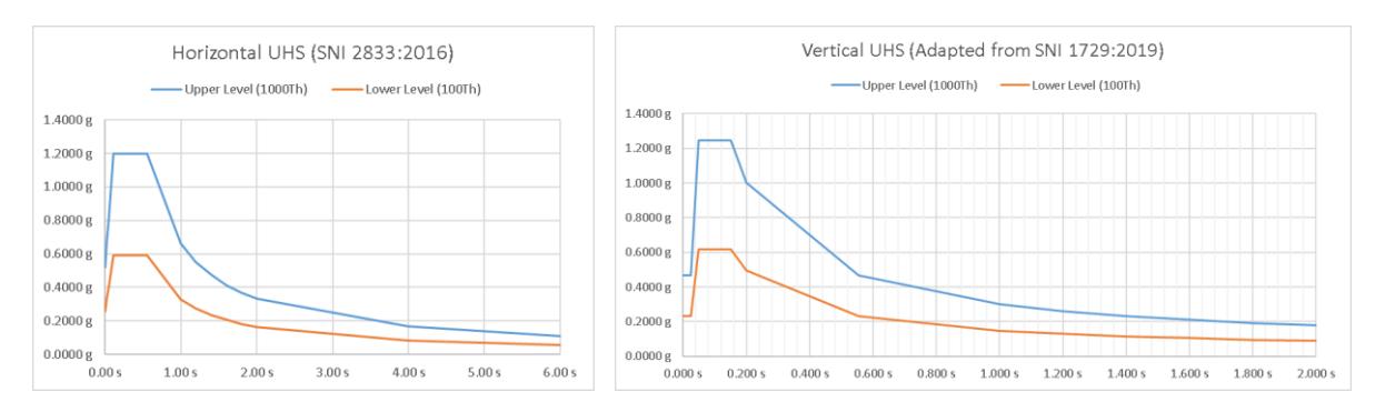
Figure 2 UHS used based on applicable standards.
Moreover, the acquisition of ground motion records involves utilizing accelerogram data tailored to the structure's location, determined by earthquake magnitude (M), distance (R), soil characteristics, spectra response form, scale factor in modification, and earthquake occurrence mechanism. A minimum of seven timehistory data sets from distinct earthquakes was employed, and the structural responses from these seven earthquakes were subsequently averaged. Notably, for structures situated in proximity to faults, critical considerations govern the selection of ground motions. Ground motions chosen for loading structures near faults necessitate pulse-like characteristics. Hayden et al. [17] and Chen et al. [18] delved into the attributes of pulse-like ground motion and its impact on structural response. Pulse-like ground motion is typified by a high amplitude and long period in the velocity time-history record.
Following the time-history selection, earthquake time-history modification was performed using the amplitude scaling method. This is imperative for bridges near faults to preserve the earthquake record's characteristics, particularly its pulse-like nature. Scaling was executed until the average response spectra of the chosen earthquake history at significant periods exceeded 85% of the predetermined target spectrum. To ensure that the characteristics remained consistent with existing earthquakes, the scale factor was constrained within the commonly used range of 0.25 to 4.00. Compliance towards the stipulated conditions is illustrated in Figure 3, which the spectrum ratio average to target spectrum of 132% for north-south and 112% east-west obtained in the scaling for the horizontal UHS at the upper level, other UHSs were scaled in the same way. The outcomes of amplitude scaling are detailed in Table 1.
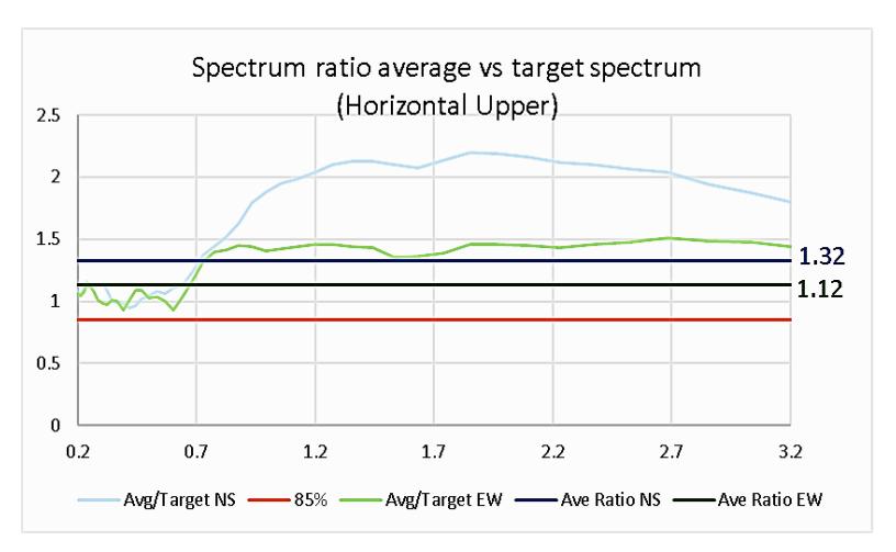
Figure 3 Example of the average ratio of spectra within the significant period.
| Scale Factor for Modification | ||||||||||
|---|---|---|---|---|---|---|---|---|---|---|
| GM | Mechanism | Earthquake | Year | Magnitude | Distance | Duration | Horizontal | Vertical | ||
| Lower | Upper | Lower | Upper | |||||||
| 1 | Shallow crust (Strike Slip) | Northridge | 1994 | 6.69 | 2.11 | 74.35 | 1.45 | 2.9 | 1.1 | 2.2 |
| 2 | Shallow crust (Strike Slip) | Imperial Valley-06 | 1979 | 6.53 | 0.56 | 36.87 | 1.5 | 3 | 1.05 | 2.15 |
| 3 | Shallow crust (Strike Slip) | Kobe, Japan | 1995 | 6.9 | 3.31 | 42 | 1.05 | 2.8 | 1 | 2 |
| 4 | Megathrust | Michoacan | 1985 | 8.1 | 83.9 | 89.41 | 1.47 | 2.94 | 1.3 | 2.6 |
| 5 | Megathrust | Peru Coast | 1974 | 7.6 | 84 | 89.41 | 1.6 | 2.9 | 1.2 | 2.45 |
| 6 | Benioff | India-Burma Border | 1988 | 7.2 | 189.9 | 85.88 | 1.45 | 2.85 | 1.2 | 2.45 |
| 7 | Benioff | Miyagi Oki | 2005 | 7.2 | 113 | 108.425 | 1.4 | 2.9 | 1.2 | 2.45 |
Table 1Ground motion used and scale factor used.
The subsequent crucial phase in implementing the Performance-Based Seismic Design (PBSD) concept is the structural analysis stage. During this phase, the author employed Nonlinear Time History Analysis, recognized for its relatively high accuracy in predicting structures' responses to seismic loads. This specific analysis was chosen due to the presence of a structural system with non-linear behavior (such as bearings and rod bars), enabling the direct capture of the structural response to the pulse-like effect of near-fault ground motion.
In accordance with ASCE 7-16 Minimum Design Loads and Associated Criteria for Buildings and Other Structures [19], the analysis involved rotating the horizontal ground motion to become parallel to the normal direction and parallel to the fault at the bridge location under examination. Additionally, the analysis accounted for the effects of vertical direction earthquakes on the bridge structure. The structural response, considered in a multidirectional context, adheres to the 100-30 rule for both earthquake directions in the loading combination.
The applicability of the performance concept hinges on ensuring the other elements' compliance with elastic behavior. Consequently, an examination of the upper structure's response to earthquake loading was imperative, encompassing both the structural capacity and the platform's response. Subsequently, after confirming the upper structure's capacity for elastic behavior, the seismic performance of the structure was ascertained following NCHRP 949 Proposed AASHTO Guidelines for Performance-Based Seismic Bridge Design [5]. This evaluation involved reviewing potential damage caused by seismic loading, utilizing engineering demand parameters generated during structural analysis, such as deformation and strain. In the context of this bridge, a critical assessment of the strain response in elements serving as earthquake-resistant components, notably the bridge pier, was conducted. The bridge's performance was then evaluated based on the specified design earthquake and the permissible level of damage to the structure resulting from seismic forces.
Results and Discussion
Model Updating Results
The outcomes of the conducted calibration revealed alterations in various structural response parameters. These encompass modifications in bridge deck geometry (Figures 4 and 5), deflection induced by static loading (Table 2), and dynamic parameters of the bridge (Table 3).
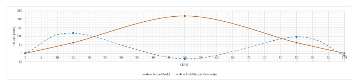
Figure 4 Comparison of model and site deck geometry before calibration.
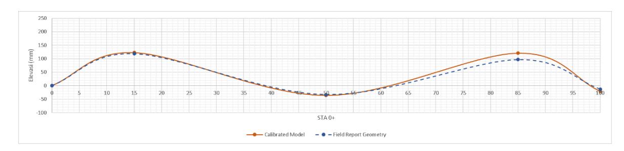
Figure 5 Comparison of model and site deck geometry after calibration.
Table 2 Comparison of static loading test results with calibrated model.
| Loading Stage | Percentage of Live Load in Loading | Mid-span D | eflection Observed (mm) | Deflection Limit (L/1000) - (mm) | |
|---|---|---|---|---|---|
| Stage | Test | Field Report | Initial Model | Calibrated Model | (11111) |
| 1 | 0% | 0 | 0 | 0 | 0 |
| 2 | 7.48% | -4 | -3.968 | -4.172 | -7.48 |
| 3 | 0% | 0 | 0 | 0 | 0 |
Table 3 Comparison of dynamic loading test results with calibrated model.
| Dynamic Load | Initial Model | ( | Calibrated Mode | I | |||
|---|---|---|---|---|---|---|---|
| Mode Shape | Test Frequency | Mode | Frequency | Period | Mode | Frequency | Period |
| (Hz) | Number | (Hz) | (s) | Number | (Hz) | (s) | |
| 1st Transversal | 0.47 | 1 | 0.376 | 2.65 | 1 | 0.391 | 2.56 |
| 1st Longitudinal | 0.98 | 2 | 0.655 | 1.52 | 3 | 0.906 | 1.10 |
| 1st Vertical | 1.62 | 9 | 1.700 | 0.58 | 8 | 1.700 | 0.58 |
Analysis of the calibration results revealed notable alterations in the geometric configuration of the bridge deck, particularly when considering the impact of shrinkage and creep of structural elements, along with modifications to element stiffness. The static test outcomes indicated that the actual structural stiffness remained relatively consistent with the initial stiffness, as the deflection results from the initial model closely aligned with the observed values.
Moreover, the calibration of the dynamic load test results demonstrated significant changes in the longitudinal direction's dynamic characteristics. These modifications, primarily focused on the existing bearing, yielded values that closely matched the observed dynamics. This calibration process is of utmost importance for structural seismic performance analysis, ensuring that the modeled structural behavior aligns with the actual conditions on the site.
Bridge Capacity Assessment Results
Adjusting the condition factor based on observations from the recent survey, determining the system factor according to the arch bridge structure, and employing a resistance factor adjusted for the forces resisted by each element, the rating factor for each element's results are presented in the tables below (Tables 4 to 7). Additionally, the calculation includes the demand capacity ratio for comparison.
Upon analyzing the results, particularly at the inventory and operating loading factor levels of the design load, it is notable that the cross girder structural element exhibited RF < 1 in its flexural capacity. This examination outcome suggests the imperative need for strengthening the element in its flexural capacity. Conversely, other elements demonstrated RF values exceeding 1, implying that they can endure maximum vehicle loads in accordance with the latest applicable regulations. This determination took into account the capacity of existing structural elements while considering the condition of each element.
In evaluating the capacity of existing structural elements, two methods were employed: the LRFR (Load and Resistance Factor Rating) and the Demand Capacity Ratio (DCR) method. The LRFR method bases its assessment on load and resistance factor calculations, incorporating a more detailed consideration of these factors. This method is sophisticated and widely adopted in contemporary engineering practice. On the other hand, the DCR method calculates the load-to-capacity ratio of the structure, providing a simpler overview but lacking detailed information about factors influencing the overall capacity of the structure.
The LRFR method is preferred in current engineering practice due to its comprehensive consideration of load and resistance factors. The results of the analysis demonstrate that calculations using LRFR yield more critical values compared to the DCR method. Consequently, for a more conservative assessment of structural elements, the LRFR calculation method is considered safer. In the LRFR method, for calculating the capacity of a structural element, particularly when dealing with concrete elements that resist axial tensile forces, such as a hanger element in an arch bridge structure, it is noteworthy that AASHTO's The Manual for Bridge Evaluation [1] lacks specific guidance for calculating the capacity rating in this context.
Table 4 Stress factor rating calculation results.
| Element | Rating Factor | |
|---|---|---|
| Hanger | Tensile Stress | 1.560 |
| Hanger | Compressive Stress | 1.746 |
| Tie Beam | Tensile Stress | 10.637 |
| не веат | Compressive Stress | 24.152 |
Table 5 Calculation results of rating factor and demand capacity ratio of ultimate flexural capacity.
| Inve | ntory | Operating | ||||||||
|---|---|---|---|---|---|---|---|---|---|---|
| Element | Demand Capacity Ratio | Rating | Rating Factor | Demand Capacity Ratio | Rating Factor | |||||
| Mx | Му | Mx | Му | Mx | Му | Mx | My | |||
| Cross | Near Support (Moment Positive) | - | 1.057 | - | 0.761 | - | 0.940 | - | 0.986 | |
| Cross Girder | Near Support (Moment Negative) | - | 0.308 | - | 2.393 | - | 0.283 | - | 3.102 | |
| Mid Span | - | 1.045 | - | 0.803 | - | 0.908 | - | 1.041 | ||
| End | Near Support (Moment Positive) | - | 0.510 | - | 3.571 | - | 0.468 | - | 4.629 | |
| Cross Girder | Near Support (Moment Negative) | - | 0.107 | - | 53.545 | - | 0.104 | - | 69.41 | |
| Mid Span | - | 0.503 | - | 3.650 | - | 0.460 | - | 4.731 | ||
| Stringer | - | 0.266 | - | 3.700 | - | 0.226 | - | 4.797 | ||
| Diaphragm | - | 0.259 | - | 16.858 | - | 0.251 | - | 21.85 | ||
| Deck Slab | 0.284 | 0.279 | 4.225 | 4.341 | 0.251 | 0.246 | 5.477 | 5.627 | ||
Table 6 Calculation results of rating factor and demand capacity ratio of ultimate axial-flexural capacity.
| Inven | tory | Opera | ting | ||||||
|---|---|---|---|---|---|---|---|---|---|
| Element | Demand Capacity Ratio | R | ating Fact | or | Demand Capacity Ratio | R | ating Fact | or | |
| Katio | Р | Му | Mz | Р | Му | Mz | |||
| Tie Beam | 0.336 | - | - | - | 0.336 | - | - | - | |
| Ri | ib | 0.706 | 3.499 | 3.822 | 4.246 | 0.676 | 4.535 | 4.955 | 5.504 |
| Hanger | Near Support | 0.486 | - | - | - | 0.478 | - | - | - |
| Mid Span | 0.504 | - | - | - | 0.487 | - | - | - | |
| Pier P3 Pier P4 | 0.076 | 48.08 | 48.29 | 109.71 | 0.003 | C2 220 | C2 C01 | 142.2 | |
| 0.076 | 1 | 3 | 9 | 0.083 | 62.328 | 62.601 | 8 | ||
| 0.076 | 48.08 1 | 48.29 3 | 109.71 9 | 0.083 | 62.328 | 62.601 | 142.2 8 | ||
| Inve | entory | Оре | erating | ||||||
|---|---|---|---|---|---|---|---|---|---|
| Element | Capacity tio | · Rating Fact | Demand Capacity actor Ratio | Rating Factor | |||||
| Vz | Vy | Vz | Vy | Vz | Vy | Vz | Vy | ||
| Tie Beam | Near Support | 0.372 | 0.372 | 5.171 | 4.980 | 0.333 | 0.334 | 6.895 | 6.577 |
| не веан | Mid Span | 0.471 | 0.424 | 3.895 | 4.329 | 0.417 | 0.380 | 5.244 | 5.736 |
| D:h | Near Support | 0.250 | 0.290 | 9.615 | 6.738 | 0.228 | 0.262 | 12.646 | 8.850 |
| Rib | Mid Span | 0.291 | 0.331 | 8.014 | 5.668 | 0.263 | 0.299 | 10.570 | 7.464 |
| Cross | Near Support | 0.268 | - | 4.578 | - | 0.223 | - | 5.935 | - |
| Girder | Mid Span | 0.276 | - | 4.199 | - | 0.226 | - | 5.443 | - |
| End Cross | Near Support | 0.153 | - | 19.288 | - | 0.142 | - | 25.003 | - |
| Girder | Mid Span | 0.173 | - | 14.957 | - | 0.159 | - | 19.388 | - |
| Chuinnan | Near Support | 0.019 | - | 66.182 | - | 0.016 | - | 85.791 | - |
| Stringer | Mid Span | 0.016 | - | 62.704 | - | 0.012 | - | 81.283 | - |
| Hanna | Near Support | 0.083 | 0.089 | 34.768 | 30.503 | 0.077 | 0.082 | 45.238 | 39.69 |
| Hanger | Mid Span | 0.114 | 0.123 | 24.790 | 21.702 | 0.105 | 0.112 | 32.305 | 28.28 |
| D: | Near Support | 0.041 | - | 2790.950 | - | 0.041 | - | 3617.898 | - |
| Diaphragm | Mid Span | 0.021 | - | 1953.776 | - | 0.021 | - | 2532.672 | - |
| Dec | k Slab | 0.326 | - | 3.065 | - | 0.252 | - | 3.973 | - |
| Pi | er P3 | 0.181 | 0.253 | 17.810 | 11.962 | 0.170 | 0.234 | 23.117 | 15.81 |
| Pi | er P4 | 0.181 | 0.253 | 17.810 | 11.962 | 0.170 | 0.234 | 23.117 | 15.81 |
Table 7 Calculation results of rating factor and demand capacity ratio of ultimate shear capacity.
Structural Performance Analysis Results
In the implementation of the seismic performance examination for structures, it is necessary to first verify the elastic behavior of structural elements that are not specifically designed for seismic resistance. Therefore, a comprehensive assessment of the upper structure's response to seismic loading is essential, encompassing both the structural capacity and the bearing response. This scrutiny is particularly crucial due to the presence of a damaged expansion joint element on the bridge. The seismic isolation system, intended to function in conjunction with the installation of high damping rubber bearings (HDRB) on the platform, may be compromised. Consequently, a comparative analysis is conducted to evaluate the impact of expansion joint damage on demand and structural response under seismic loads. The results of this comparative analysis are depicted in the graphs (Figures 6 and 7) and summarized in Table 8 below, providing insight into the effects of damaged expansion joints on demand and structural response due to seismic loads.
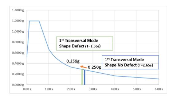
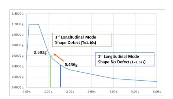
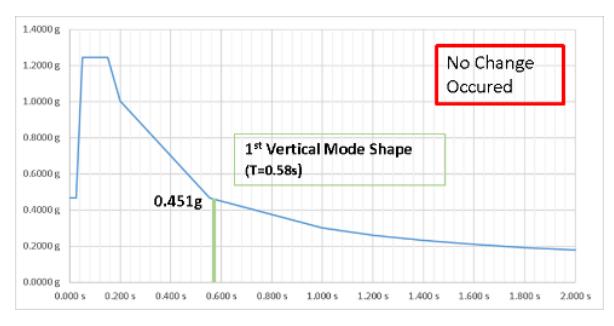
Figure 6 Changes in seismic demand due to expansion joint defects.
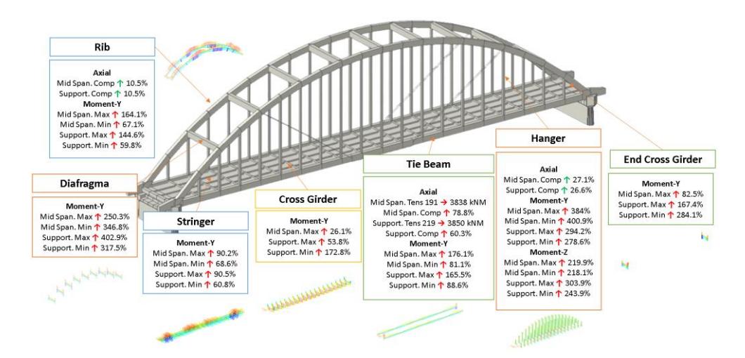
Figure 7 Changes in force due to expansion joint defects.
Table 8 Changes in upper structure demand capacity ratio due to expansion joint defects.
| Defect | No Defect | ||
|---|---|---|---|
| Element | Demand Capacity Ratio | Demand Capacity Ratio | |
| My | My | ||
| Near Support (Moment Positive) | 0.868 | 0.728 | |
| Cross | Near Support (Moment Negative) | 0.692 | 0.375 |
| Girder | Mid Span | 0.702 | 0.679 |
| End | Near Support (Moment Positive) | 1.124 | 0.651 |
| Cross | Near Support (Moment Negative) | 1.051 | 0.454 |
| Girder | Mid Span | 0.594 | 0.457 |
| Stringer | 0.432 | 0.349 | |
| Diaphragm | 2.165 | 0.867 | |
| Tie Beam | 0.921 | 0.582 | |
| Rib | 1.050 | 0.755 | |
| Near Support | 2.283 | 0.911 | |
| Hanger | Mid Span | 1.314 | 0.801 |
The analysis results concerning seismic demand indicated a notable increase in the seismic demand along the longitudinal direction, approximately 1.38 times higher. This suggests an escalation in the response of the bridge's structural elements should be anticipated. The presence of defects, specifically the damaged expansion joints, imposes a constraint on the superstructure system, which is designed to freely expand above the existing support with the isolation system. As a consequence of this limitation in longitudinal motion, the seismic force resisted by the superstructure elements increases, resulting in some elements experiencing a demand surpassing their capacity. Consequently, the existing elements cannot be assured to remain elastic. Therefore, it is crucial to address the damage to the expansion joints before conducting a performance inspection. Rectifying this issue is paramount to restoring the flexibility of the superstructure elements, ensuring that they can adequately respond to seismic forces while remaining within their elastic limits.
In addition to ensuring the condition of the upper structural elements, it is crucial to assess the potential for overturning in tall bridges, such as arch bridges. This involves verifying that the bearings do not experience axial tensile forces in the vertical direction during seismic loading. The potential for overturning, if not addressed, poses a significant risk to the stability of tall structures. Moreover, it is essential to consider the potential for pounding on the bearings. Ensuring that there is adequate space within the bearing area with the existing gap is vital to prevent pounding. Pounding refers to the collision or impact between adjacent structural elements during seismic events, which can lead to severe structural damage. Thus, maintaining sufficient clearance within the bearing area is critical to mitigating the risk of pounding and ensuring the overall seismic resilience of the bridge structure.
| Bearing Displacement Check (No Defect) | ||||||||
|---|---|---|---|---|---|---|---|---|
| Displacement Relative (m) | ||||||||
| Bearing No. | X dir. (Longitudinal) | Y dir. (Transversal) | Resultant | |||||
| 1 | 0.1534 | 0.1259 | 0.2333 | |||||
| 2 | 0.1542 | 0.1268 | 0.2342 | |||||
| 3 | 0.1584 | 0.1259 | 0.2362 | |||||
| 4 | 0.1576 | 0.1268 | 0.2364 | |||||
Table 9 Displacement of the bearings with the assumption that there is no damage in the expansion joints.
Upon assessing the displacement at the bearings, presented in Table 9, it is observed that the available gap on the bridge for accommodating displacement is 5 cm (0.05 m) longitudinally and 10 cm (0.1 m) transversely. This discrepancy raises concerns about potential pounding during an earthquake, jeopardizing the intended isolation of the structural system. This aspect must be thoroughly considered in the rehabilitation plan before incorporating the results from the existing seismic performance analysis.
Once the superstructure's elastic behavior is confirmed and measures are in place to prevent pounding in the bearing, the outcomes of the seismic performance analysis based on the NCHRP 949 document can be employed. Within the performance analysis, the strain of the concrete and reinforcement elements on the bridge pier is a critical engineering demand parameter (EDP) used to assess the structure's performance. The maximum strain recorded serves as a determinant for the existing structure's performance level, as outlined in Table 10.
Table 10 Strain limits and their relationship with performance levels as per NCHRP 949.
| Engineering Design | Performance Level | |||||||
|---|---|---|---|---|---|---|---|---|
| Parameters | PL1: Life Safety | PL2: Operational | PL3: Fully Operational | |||||
| Reinforcement tensile strain limit (RC Column) | 𝑓𝑦ℎ𝑒 𝑃 𝜀𝑠𝑏𝑢𝑐𝑘𝑙𝑖𝑛𝑔 𝑏𝑎𝑟 = 0.032 + 790𝜌𝑠 − 0.14 𝐸𝑠 𝑓′𝑐𝑒 𝐴𝑔 | 𝜀𝑠 𝑏𝑎𝑟 = 0.8𝜀𝑠𝑏𝑢𝑐𝑘𝑙𝑖𝑛𝑔 | ≤ 0.010 | |||||
| Concrete compressive strain limit (RC Column) | 𝜌𝑣𝑓𝑦ℎ𝜀𝑠𝑢 𝜀𝑐 = 1.4 (0.004 + 1.4 ) 𝑓′𝑐𝑐 | 𝜌𝑣𝑓𝑦ℎ𝜀𝑠𝑢 𝜀𝑐 = (0.004 + 1.4 ) 𝑓′𝑐𝑐 | ≤ 0.004 | |||||
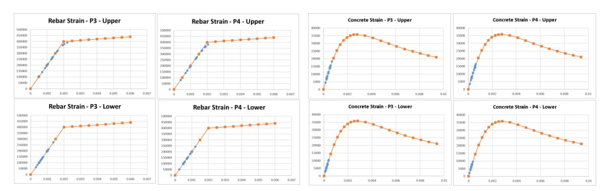
Figure 8 Strain that occurs due to seismic loading.
The results of the examination of the strain on the bridge column, illustrated in Figure 8, indicate that the strain levels remained within the elastic region for both concrete and steel reinforcement. Consequently, the performance of the bridge is categorized as fully operational. In accordance with the guidelines outlined in the FHWA's Seismic Retrofitting Manual for Highway Structures. Part 1 Bridges document [20], this bridge is not prioritized for seismic retrofitting of its columns.
Beyond the performance analysis, an additional phenomenon discerned from this investigation is the impact of employing pulse-like ground motion on the structural response. The non-linear time history analysis conducted enables the visualization of the structural response for each time-step under the applied seismic loading. The observations presented in Figure 9 and Table 11 reveal that the maximum structural response coincides with the time step where a pulse-like phenomenon is evident in the velocity time history of the seismic input. This underscores the significance of utilizing ground motion with pulse-like characteristics, particularly for structures located near faults, as it exerts a notable influence on the structural response.
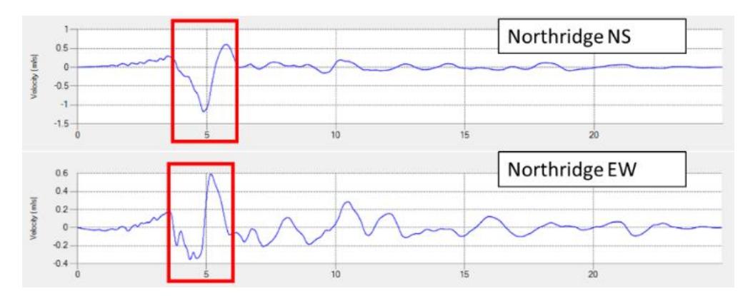
Figure 9 Velocity time history with pulse-like characteristic.
Table 11 Maximum structural response and time-step at which it occurs.
| Max Base Shear Y | Max Base Shear Z | ||||
|---|---|---|---|---|---|
| Ground Motion | Force (Kn) | Time Step | Force (Kn) | Time Step | |
| Northridge NS | 1312.71 | 5.00 | 6653.01 | 4.75 | |
| Northridge EW | 4052.00 | 5.00 | -2131.38 | 4.70 | |
Conclusion
In conclusion, the calibration of the finite element model (FEM) plays a crucial role in influencing the accuracy of the calculations, impacting service loading capacity and seismic analysis. Calibration led to changes in stiffness and time-dependent material effects, notably a 1.38-times increase in longitudinal earthquake demand when compared to the uncalibrated model. This indicates that model updating significantly affects the response of the structure towards the applied loads.
Furthermore, both the Load & Resistance Factor Rating (LRFR) and the Demand Capacity Ratio (DCR) method is viable for assessing structural element capacity. LRFR calculations yield more critical values, making it a safer choice for a conservative assessment. However, LRFR lacks specific guidance for rating the capacity of concrete elements resisting axial tensile forces.
Additionally, this study recommends the utilization of ground motion with pulse-like characteristics for seismic loading near faults due to its significant impact on the structural response. The performance concept is applicable with the prerequisite that other elements remain elastic. Defects in expansion joints can increase forces resisted by upper structural elements, necessitating priority repairs. Pounding potential on the bearings must also be addressed to align with analysis results based on NCHRP 949's guidance.
The conducted case study provided bridge condition assessment results, capacity assessment using LRFR reveals critical stresses, such as tensile stresses in the hanger elements (1.560) and flexural capacity in the cross girder elements (0.761 for the inventory design level, 0.986 for the operating design level). This implies a need to enhance the flexural capacity of the cross girder structural elements. The strain assessment on the piers indicates that the bridge meets the fully operational performance level at both upper and lower hazard levels. However, considerations include potential upper structure damage due to expansion joint issues and the risk of pounding on the bearings during seismic events. The results obtained are sufficient to justify structural retrofit to maintain the service life of the bridge structure.
Nomenclature
= Rating factor
= Capacity
= Allowable stress
= Nominal resistance of the element (, , or )
= Dead load
= Super-imposed dead load
= Permanent load beside dead load and super-imposed dead load, i.e., prestress load
= Live load
= Dynamic load factor, = 50 +125 ≤ 0.30 with L in ft
= Dead load factor
= SIDL factor
= Factor for permanent load beside dead load and super-imposed dead load (prestress load, creep and shrinkage load) = 1.0
= Live load factor
= Structural element condition factor
= Structural system factor
= Structural resistance factor according to LRFD document