
Introduction
Active fault zones are primarily identified by the presence of earthquakes along with evidence of surface deformation. When a fault surface rupture is detected, it is delineated as a line and assigned a buffer zone along that line with a specific radius, representing the area potentially experiencing further deformation. Thus, the foundational information for mapping active fault zones is derived from fault surface rupture, which prompts the question of how to define the active fault zone when fault surface rupture cannot be found or tracking it is impractical. An example of this scenario is seen in the Baribis Fault mapped by Aribowo et al. in [1], where the fault surface rupture ends on the eastern side of southern Jakarta, while in 1780, an earthquake with a magnitude of more than 8.5 Mw (estimated by Albini et al. in [2] and Nguyen et al. in [3]) was recorded. The conventional assumption in earthquake science, which has been challenged by Hamling et al. through their 2016 Kaikoura earthquake findings, is the belief that earthquakes are typically confined to a single fault or a predictable fault segment. The research by Daryono et al. in [4] has further complicated this view, showing that fault lengths alone may not be reliable indicators of earthquake magnitude, as multifault ruptures can occur. Additionally, sandbox modeling, a method used to simulate geological processes, indicates that an earthquake event is highly likely to produce multiple surface ruptures. These findings collectively suggest a need for revising our understanding of earthquake dynamics and seismic risk assessment. This raises questions about the actual termination point of fault surface ruptures and the possibility of defining active fault zones solely based on seismic data without considering fault surface rupture.
Fault surface rupture manifests itself on the surface of sedimentary rocks due to the movement of crystalline rocks (igneous and metamorphic) beneath them along fault planes. Crystalline rocks and sediments display differing mechanical behaviors (rheology), leading to distinct deformation kinematics. For instance, in regions where brittle deformation regimes prevail, folds in sedimentary rocks are observable, in contrast to crystalline rocks. Crystalline rocks, integral to actively moving plates, undergo deformation, culminating in seismic events. Hence, in this context, sedimentary rocks typically assume a passive role in fault surface rupture formation events. The propagation of buried fault to the surface is reflected in surface movements, a phenomenon that can be examined through analogue sandbox modeling.
InSAR is particularly well-suited for measuring ground displacement associated with earthquakes, as explained by Massonet et al. in [5] and Bürgmann et al. in [6]. By comparing pre- and post-event radar images, InSAR can generate interferograms that reveal the surface deformation caused by an earthquake. These interferograms can determine the amount and direction of ground movement, providing valuable insight into an earthquake's faulting mechanism, slip distribution, and surface rupture extent. Surface rupturing occurs when the displacement along a fault extends to the Earth's surface. Also, InSAR data can map active faults and monitor crustal deformation over time. Studying earthquake processes and fault system behavior is crucial for understanding the risks associated with seismic hazards. Post-earthquake Interferometric Synthetic Aperture Radar (InSAR) observations of surface movement have provided valuable insight into crustal deformation and fault movement during earthquakes. Bekaert et al. in [7] explains that one of the challenges in InSAR interpretation is the ambiguity in determining fault geometry and slip distribution, not to mention issues related to atmospheric effects and interferometric phase errors. However, closer examination of the relationship between InSAR observations and analogue models is needed to better understand the complex processes involved in earthquake generation. The present research explored the correlation between InSAR earthquake observations and analogue sandbox modeling.
Analogue sandbox modeling is a well-established experimental method used in geology and geophysics to simulate and understand complex geological processes, including faulting, folding, and the evolution of sedimentary basins and mountain ranges, as previously studied by Sapiie et al. in [8] and [9] and extensively reviewed by Graveleau et al. in [10]. In a typical sandbox experiment, layers of granular materials (i.e., sand) represent the Earth's crust, as previously studied by Lohrmann et al. in [11] and Reber et al. in [12]. These layers are deformed by applying forces that mimic tectonic stresses, enabling the researchers to observe the resulting structural patterns and deformation processes. The properties of the granular materials, the configuration of the layers, and the applied boundary conditions can be varied to simulate different geological scenarios and crustal conditions. High-resolution images are taken throughout the experiments and particle image velocimetry (PIV) analysis is used to calculate the particle displacement in the sandbox experiments, enabling the quantification of surficial movement patterns. The PIV data can be statistically analyzed to identify key trends and relationships between fault kinematics and surficial movement patterns, as previously studied by Adam et al. in [13], Cruz et al. in [14], Dotare et al. in [15], Marshak et al. in [16].
This research constitutes a preliminary study to demonstrate PIV analysis of sandbox experiments as an approach for investigating surface deformation and surface rupture patterns on the Earth's surface between earthquake cycles, which may be compared to surface displacement data such as InSAR or GPS observations. Furthermore, this study aimed to uncover the relationship between fault kinematics and surficial movement patterns of earth crust deformation.
Earthquake Nucleation and Cycles
Iio in [17] explains that earthquake nucleation begins when an earthquake begins, marked by the initial rupture along a fault within the Earth's crust. Fundamentally, it involves the transition of a fault from a state of stability to rapid slip. This process is influenced by the complex structural evolution of faults, which begin as fractures in intact rock volumes and develop into distinct zones of weakness that can accommodate slip. The nucleation phase is typically characterized by a gradual accumulation of stress on the fault until it exceeds the rock's strength, leading to sudden displacement. This critical transition is governed by factors such as the physical properties of the fault zone, the ambient stress field, and the history of previous seismic activity. The precise
mechanisms that trigger the onset of rapid slip remain a subject of ongoing research, with various models suggesting different combinations of factors like fluid pressure, aseismic slip, or mechanical instabilities.
Earthquake cycles, a well-documented geological phenomenon, involve a repetitive pattern of seismic activity along fault lines, spanning decades to centuries, depending on the earthquake's magnitude. These cycles comprise three distinct phases:
- 1. Inter-seismic slip, characterized by gradual strain accumulation and fault frictional locking,
- 2. Co-seismic slip, marked by sudden rupture during an earthquake event,
- 3. Post-seismic slip, occurring over minutes to years as the crust and fault adjust to altered stress conditions.
These cycles manifest themselves across various fault types. While the concept of seismic cycles posits that stress accumulates on a fault before being swiftly released in a major earthquake, its verification remains challenging due to the infrequent occurrence of large earthquakes and the influence of nearby seismic events on the stress dynamics.
A profound discrepancy exists in spatial and temporal scales between real-world observations and sandbox models (Figure 1). Sandbox experiments, often used to simulate seismic cycles, can compress several cycles into a pair of time-lapse photographs. On the other hand, this contrasts with InSAR techniques in real-world seismology, which typically capture changes between pre-seismic and co-seismic conditions. To bridge this gap requires photographic acquisition at the shortest feasible intervals in sandbox models that aim to mimic the duration of a single seismic cycle more accurately. This approach, however, faces limitations due to the resolution capabilities of the camera and the data processing constraints of particle image velocimetry systems. As the intervals between time-lapses reduce, the magnitude of model displacement decreases, potentially increasing noise interference in the data. This approach necessitates a careful balance, possibly through enhanced imaging technologies or advanced noise filtration methods, to ensure that the data captured is representative and reliable. By integrating such improvements, researchers can better align sandbox models with real-world seismic data, offering more precise insight into earthquake dynamics.
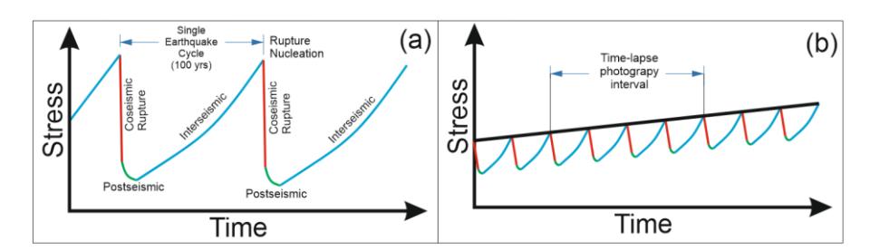
Illustration of seismic cycle in (a) real world and (a) model perspective.
Sandbox Modeling
This study performed sandbox modeling experiments to investigate three primary fault systems: reverse faults, normal faults, and strike-slip faults. All experiments used homogenous sifted sand, deformed with a consistent shortening velocity of 5 cm/hr, with a 15-second time-lapse interval for photography. PIV analysis was performed on the entire series of time-lapse photos generated.
To model a reverse fault, instead of directly pushing sand using an indenter (thin-skin deformation, as studied by Hubbert et al. in [18] and Dahlen et al. in [19]), we employed a rigid block pushed by an indenter to induce vertical movement (thick-skin deformation, as studied by Lacombe and Bellahsen in [20] and Pfiffner in [21]). For strike-slip faults, we utilized planar plates that move past each other, as investigated by Visage et al. in [22]. Lastly, normal faults in sedimentary rocks develop due to fault propagation resulting from vertical movement in crystalline rocks. This movement in crystalline rocks is triggered by tensile forces acting on the plates. Pulling a mica sheet beneath the sand layer allowed us to simulate the tensile forces acting on the sand layer, without using a rigid block (see review by McClay in [23]).
Modeling Material
Schreurs et al. in [24] found significant variability in experimental results across laboratories despite using the same types of quartz sand and corundum. This variation was mainly due to minor differences in how the sand was handled and stored, affecting the bulk density of the material. Factors like the height of sand sieving, sieving speed, and techniques for removing excess sand could cause slight differences in bulk density, subsequently affecting the mechanical properties of the sand. These minor changes in sieving height and speed may lead to lateral and vertical differences in peak and boundary friction angles and cohesion values of the material after model construction. Initial differences in basal friction were considered significant in causing model variability, indicating the sensitivity of sand's frictional behavior to slight variations in material state or experimental setup. This complexity makes it challenging to translate quantitative outcomes like the number of thrusts, the distance between thrusts, and the width of pop-up structures from models to natural phenomena.
Based on the survey of Klinkmuller et al. in [24], involving 14 analog sandbox modeling laboratories, the reproducibility of sandbox experiments in geoscience modeling depends on various material properties, such as grain size, shape, material homogeneity, and moisture content. Variations in grain size and shape can lead to differences in the model's frictional properties and packing densities, ultimately affecting its mechanical behavior. Ensuring uniformity in material composition is crucial to maintaining consistent behavior throughout the model, as deviations can introduce unpredictability. Additionally, moisture content plays a significant role, altering the mechanical properties of granular materials and potentially causing variations in experimental outcomes. Standardized measurement and reporting methods are essential to enhance reproducibility, providing a solid foundation for assessing and comparing experiment results.
We employed natural sand sourced from the Ngrayong Formation in East Java to enhance the reproducibility in our experimental design. This particular sand is characterized by a high quartz grain content, ranging from 90- 95%, which ensures a high degree of homogeneity. We sifted the sand through a #80-mesh sieve to obtain precise surface deformation details. This sieving process is crucial, as it contributes to creating distinct and sharp deformation features on the surface. In contrast, utilizing a coarser grade of sand, for example passed through a #50 mesh, would result in less pronounced surface details, leading to only subtle surface cracks and folds, thereby obscuring finer deformation characteristics. Additionally, we implemented a coloration technique to the sand to facilitate direct visual observation of the cross-sectional side, enhancing the clarity and effectiveness of our observations.
In our experiments, we chose to use a sand layer with a thickness of 8 cm, a decision informed by the balance between theoretical advantages and practical limitations. Thicker layers, as we have observed, offer a wider observational area, enabling more comprehensive tracking of the deformation processes. This setting is crucial for accurately analyzing the evolution of strain patterns in the material. We also had to consider the capacity of our equipment. For example, overly thick layers beyond 15 cm could strain our machinery, resulting in uneven stress application. By comparing these practical constraints with our need for detailed data, we concluded that an 8-cm layer would strike the optimal balance.
PIV Analysis
Particle image velocimetry is an indirect measurement method from a pair of images by dividing the image into hundreds of columns and rows, forming an array of cells (see review by Adrian and Westerweel in [25] and Raffel et al. in [26]). Each cell is known as an interrogation window (IW). Typically, the size of these IWs can range from 16 x 16 pixels to 128 x 128 pixels, depending on the size of the analyzed image and the desired level of detail density. Cross-correlation is performed on each IW, after which the displacements are calculated for each. Finally, a displacement field map with individual pixels representing the IW is produced.
The configuration settings for this analysis are presented in Table 1. The choice of IW size has implications for operation speed and detailed information. Larger IW sizes result in faster operation and smoother outcomes but may sacrifice detailed information. Conversely, smaller IW sizes provide more detailed results but may lead to slower operation and a higher likelihood of generating artefacts. Ideally, the IW size must be larger than the magnitude of maximum displacement (in pixel units). Therefore, we have to find the IW size for a given image dimension size to achieve optimum quality.
Table 1 PIV settings applied in this study.
| Step | Operation | Note |
|---|---|---|
| 1 | image loading | Image sequence using .jpg format |
| 2 | ROI | Whole image area |
| 3 | Pre-processing | CLAHE for contrast enhancement Especially for side views, high pass filter is enabled |
| 4 | Analysis | FFT, 3 Pass (64 px, 32 px, 16 px) |
Before performing the PIV analysis, we applied high-pass filtering preprocessing to the analyzed images to remove artefacts from PIV miscalculations. In the cross-sectional view images, the layering of colors provided a very high contrast compared to other regions that did not exhibit layering. Therefore, artefacts were produced along the layer boundaries in the PIV analysis results.
To visualize the PIV results, we color-coded the displacement field map and generated a movement vector using an arrow to indicate the direction of movement. From displacement field data, we calculated shear strain rates (1 and 2) and vorticity (3) using equations from Meynart in [27] and Yan et al. in [28]:
\[\frac{dV}{dX} = \frac{V(1+1,j) - V(1-1,j)}{X(1+1,j) - X(1-1,j)} \tag{1}\]
\[\frac{dU}{dY} = \frac{U(i,j+1) - U(i,j-1)}{Y(i,j+1) - Y(i,j-1)} \tag{2}\]
\[\Omega = \frac{dV}{dX} - \frac{dU}{dY} \tag{3}\] where U and V represent the velocity components in the X and Y directions of the PIV system, respectively.
By default, the produced displacement field maps are in pixel units. Therefore, calibration is necessary to convert the displacement vectors into real-world units. Dividing the total length shortening (or extension) applied by the number of frames will provide the magnitude of the maximum displacement observed in the experiment. This ratio is then used to convert the pixel units to mm or cm.
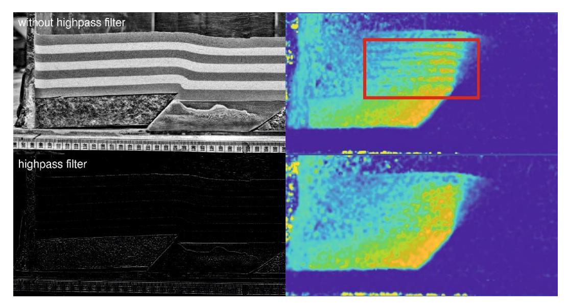
Using a high-pass filter in the preprocessing stage can help eliminate artefacts in the PIV analysis results caused by the high color contrast of the layered regions. By applying a high-pass filter, the low-frequency components associated with the layered colors can be attenuated, which helps to enhance the accuracy and reliability of the PIV analysis by reducing the impact of artefacts and improving the quality of the displacement field obtained from the images.
Active Rupture Zone Length Analysis
As previously explained, the displacement field can be used to calculate its displacement gradient, which indicates the active rupture zone. This concept applies to both plan and cross-sectional views. The active rupture zone's length can then be measured and the results can be plotted against the applied cumulative strain. Our hypothesis posits that the changing pattern of active rupture length reflects the dynamics of related fault development activities. Typically, rupture traces begin as isolated zones. With increasing strain, the length of the rupture activity zone may either expand or contract, representing how faults behave under continued deformation. It is essential to note that when rupture activity ceases, the fault rupture trace remains and does not disappear. During rupture activity, fault rupture traces form, indicating the lengthening of the active rupture zone in previously undeformed material. Eventually, as this activity diminishes or stops, meaning its length shortens, the traces from earlier activity persist. Therefore, it is crucial to distinguish between rupture activity length and rupture trace length.
From Nature to Model
In order to accurately produce a proper sandbox model that depicts real-world conditions, one must scale the real-world settings to the model. Four aspects need to be considered: stress configuration, amount of strain, and geometric and time scaling, which are translated into basement setting, indenter shape, type (shortening or tensional) and direction of stress, strain amount, and rate, material to be used, thickness, and stratigraphic setting. Failure to honor these aspects may produce an unreliable model.
How thick and how extended should the sand in the model be? First, we need regional geologic cross-sections for reference. The more, the better. We tried to match the aspect ratio of the natural case to the model. Usually, the longer the line to model, the thinner the total thickness of the model. Principally, sandbox modeling is about deforming sand. The first assumption is that the stratigraphy of the research area is analogous to 100% sand. Usually, a complete package of sand gives acceptable results. Suppose the faults' or folding height's spacing significantly differs from the natural case. In that case, we can add gypsum or glass bead layers within the model stratigraphy according to the study area stratigraphy.
The combination of the basement rock setting that underlies sedimentary rocks and the setting of tectonic forces held information for designing the stress configuration for our model. The distribution and pattern of the strike of faults and folding axis may reflect the basement configuration. Generally, we can infer the direction of the tectonic force by taking a perpendicular line from the strike of the folding axis if a seismic survey is unavailable. In order to produce a series of thrust and reverse faults, we can introduce stress perpendicularly. If a strike-slip fault is found in the area of study, we can apply oblique convergence (simple shear deformation) instead of applying perpendicular convergence. We can introduce basement anisotropy to model lateral strike changes, such as a high basement or a high friction layer (i.e., sandpaper) within the model. In general, for normal fault systems, the same applies as explained above. Normal faults are produced by applying tensional forces by moving the indenters away from each other.
Now that the model has been constructed, how do we deform the model? Principally, there is no connection between the shortening rate and the Hookean deformation law. In nature, the deformation rate affects the change in the deformed material (i.e., heat transfer and diagenesis). Since there is no change in material properties during the sandbox experiment, we can neglect the rate of indenter movement. Usually, we use the slowest possible rate of indenter movement to prevent undesired deformation, such as cracking, in the produced model. In order to estimate how much strain has to be applied, we can perform a palinspastic analysis of the reference geologic cross-section. Thus, the total strain is obtained.
Results
Reverse Fault
At the onset of the experiment, observations in both cross-sectional and planar views revealed a gradual reduction in displacement magnitude toward the foreland, indicating a progression of strain. The deformation front systematically moves toward the foreland, stopping near the future surface rupture zone, signifying the initiation of blind fault development. As the blind fault advances, the displacement magnitude of the hanging wall steadily increases until a fault surface rupture becomes apparent – subsequently, a regional fold with a shallow dip is formed above the basement fault within the sand layer.
Following the fault surface rupture, the hanging wall experiences displacement with a constant magnitude. The hanging wall's movement extends beyond the anticipated fault surface rupture in both planar and crosssectional perspectives preceding the surface rupture. The maximum displacement magnitude is observed at the hanging wall's edge near the expected fault surface rupture, gradually diminishing toward the hinterland portion of the hanging wall.
Fault propagation initiates at the basement contact with the sand layer and progresses gradually until breaching the surface, as evident in the cross-sectional view. Initially, a short-length fault emerges above the basement contact with the sand layer, giving rise to folding above it. Suddenly, the fault extends to the surface, resulting in a fault surface rupture. The central portion of the model tends to generate fault surface rupture much earlier than the region adjacent to the glass wall. Consequently, fault surface rupture propagates laterally outward from the model's middle part. This phenomenon is attributed to the friction between the sand and the glass wall, which increases resistance to fault production (Figure 3).
Illustration of fault surface rupture formation compared to fault progression at depth of blind fault development (left: horizontal displacement field map, right: displacement gradient map derived from the displacement map).
Our measurements revealed that fault ruptures, both on the surface and subsurface, exhibit an exponentially increasing velocity (Figure 4). Initially, the surface rupture emerges and extends towards the model's perimeter. Cross-sectional analysis displayed a gradual rupture propagation, marked by two ruptures that merge at a total strain of 14.1 mm. The subsurface rupture forms at a steeper angle than the 50° dip of the basement fault. With increasing strain, this angle becomes even more pronounced.
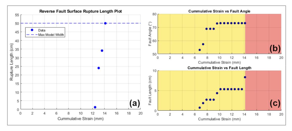
(a) This plot illustrates the swift lateral propagation of the surface rupture observed at plan view, with notable lengthening at minor strain increments. The blue dashed line indicates a physical barrier in the model, preventing further propagation. (b) This plot demonstrates that the fault's dip angle exceeds the 50° angle of the basement observed in the cross-sectional view. (c) This plot indicates a steady augmentation in fault length corresponding to the cumulative strain observed in the cross-sectional view. Any increase in strain beyond the yellow zone does not indicate a change in fault surface rupture geometry and length.
Strike Slip Fault
Strike-slip fault movement is initiated by two plates moving beneath the sand layer, accumulating strain on the surface. The zone where strain accumulates is denoted by an area with no movement, depicted as the colorless central part of the model. Employing a pair of square plates moving parallel to each other in our model, the sand is displaced in parallel with comparable velocities of both plates, leading to the emergence of a non-moving zone between them. This non-moving zone signifies the strain accumulation area responsible for surface deformation.
At the onset of deformation, the non-moving zone (NMZ) is distributed along the anticipated primary deformation zone (PDZ) (Figure 5). A detailed examination of the NMZ surface revealed the rotation of the square marker, with the fault surface rupture yet to be generated. As deformation progresses, the NMZ gradually contracts, giving rise to a series of en-echelon surface ruptures between NMZ segments, which denote the development of pop-up structures (Figure 6). Simultaneously, the termination of the surface rupture line assumes a curved form, delineating the boundary of the pop-up deformation. With increasing shortening, the NMZ continues to narrow and en-echelon surface ruptures progressively connect, forming a single fault. This gradual process persists until each en-echelon surface rupture coalesces into a unified PDZ.
Measurement of the active rupture zone length of strike-slip fault segments prior to the formation of the PDZ shows that the length of the rupture in each segment increased at a constant rate. Segments 1 and 3 formed first, followed by segments 2 and 4. All segments were uniformly oriented, forming a 10° angle with the direction of the applied force. A subsequent decrease in movement activity on these ruptures was observed a moment before the merging of two fault segments. The merging process of the segments into the PDZ is reflected in the changes in the length of the active fault surface rupture.
The accumulation of strain in the middle part of the model. At the initial stage of surface rupture development, regularly spaced en-echelon faults are formed, distributed following the shape of the basement discontinuity. The principal deformation zone (PDZ) is formed through the gradual anastomosis of en-echelon fault arrays.
The internal cross-section of the middle part of the model shows the formation of pop-ups.
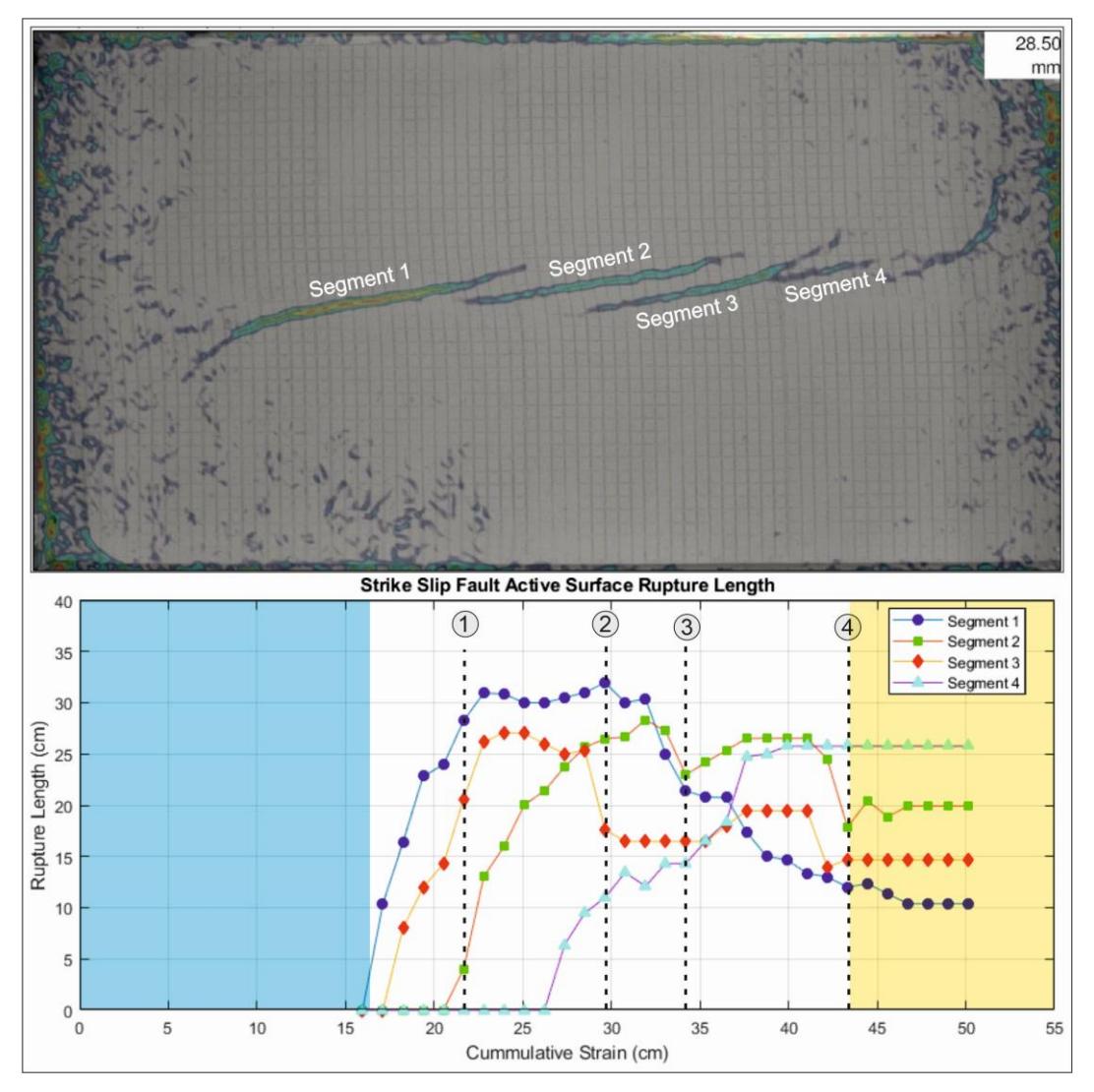
The development pattern of the length of the active surface rupture. The blue zone indicates events without fault surface rupture. Event 1 marks the initial formation of segment 2. In event 2, segments 4 and 3 as well as segments 2 and 1 merge. By event 4 (the yellow zone), the PDZ is fully formed and enters a steady state.
Normal Fault
The formation of a normal fault (NF) is driven by applying tensile forces, resulting in extensional deformation. These tensile forces are applied to the detachment sheet, causing the material above it to move simultaneously. We used a rigid basement block with a listric shape, which controlled the deformation of the material above it when the detachment sheet was pulled.
Different types of normal faults form within this context. The primary normal fault (PNF) is the normal fault that forms above the listric basement block, dipping in the direction of the applied tensile forces. The movement of the PNF causes the rotation of the material above it, leading to the formation of new normal faults. These newly formed normal faults are defined based on their dip direction: those dipping in the same direction as the PNF are called synthetic normal faults, while those dipping in the opposite direction are called antithetic normal faults. The first fault to form after the PNF is an antithetic PNF (PNFa) at the farthest end of the model, followed by a major synthetic normal fault (MNF), which formed between PNF and PNFa. Additional faults are formed between PNF and PNFa, including the major synthetic normal fault (MNF) and a major antithetic NF (MNFa). The MNF emerges immediately after PNFa, followed by MNFa, and then the minor normal fault (mNF) forms simultaneously along normal fault surface rupture development.
The active rupture zone analysis revealed intricate details about normal fault dynamics. We analyzed two antithetic PNFs (PNFa-1 and PNFa-2), an MNF, and its antithetic normal faults (MNFa 1-3). PNFa-1 formed initially due to accumulated extensional strain in the material. As the strain continued to increase, PNFa-2 developed concurrently with the development of PNFa-1. Interestingly, the emergence of PNFa-2 coincided with a decrease in the length of PNFa-1, leading to an eventual reduction in PNFa-1's activity and its replacement by PNFa-2. This process resulted in the imbrication of the two antithetic PNFs. The active rupture zone of the MNF formed shortly after the development of PNFa-1. Throughout the deformation process, the MNF remained continuously active, with its active rupture zone length gradually extending to the lateral limits of the model. A notable decrease in the MNF's activity was observed following the formation of its MNFa. The formation of MNFa's occurred at three distinct locations: two near the model's walls (MNFa-1 and MNFa-3) and one in the middle (MNFa-2). These faults exhibited different movement patterns. MNFa-1 and MNFa-3 did not show significant development, with MNFa-1 being briefly active. In contrast, MNFa-3 remained active until the end of the experiment, likely influenced by its proximity to other faults. MNFa-2, however, developed significantly and was active over a prolonged duration. A decrease followed the cessation of MNFa-2's activity in the MNF's activity. Overall, the active rupture zone of the observed faults displayed an intermittent activity pattern and a marked departure from the continuous activity pattern typically seen in contractional experiment settings, highlighting
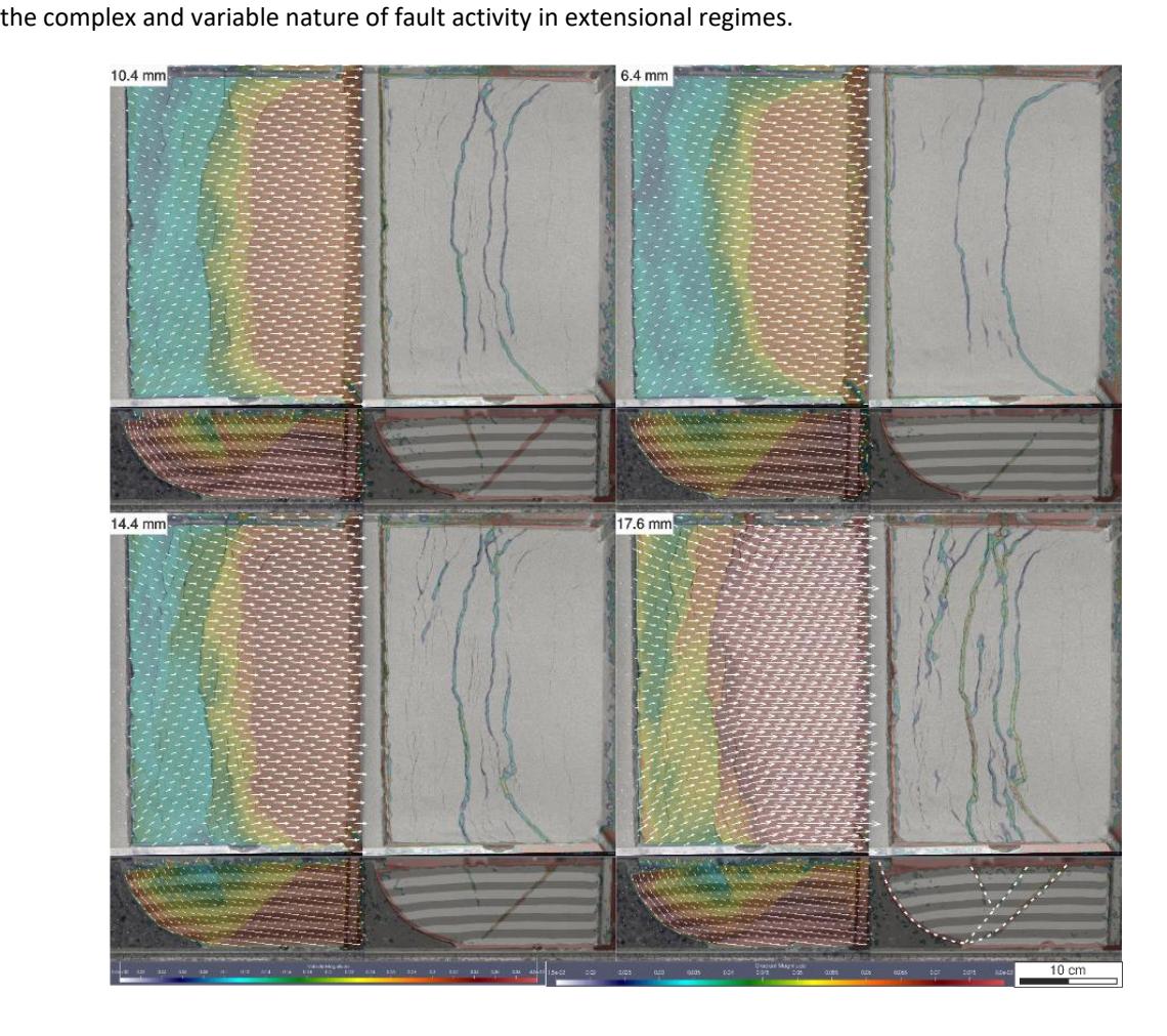
The development of normal faults in this model exhibited high movement patterns in the indenter region and weakened around the main fault. The distribution of faults extended from the central part of the model towards the main fault. Systematically, the antithetic main normal fault developed in an imbricated manner as strain increased, followed by the development of minor normal faults.
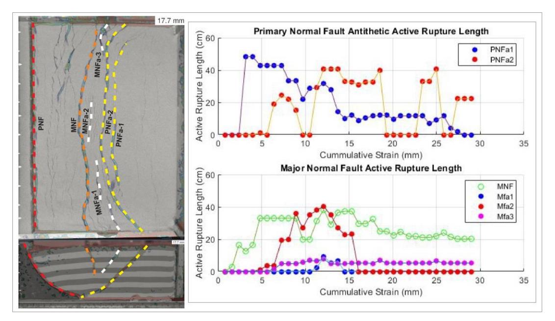
Analysis of active rupture zones in normal faults revealed dynamic interactions: PNFa-1's activity diminished with the emergence of PNFa-2, while the MNF remained consistently active with variable development in its antithetic faults MNFa 1-3, illustrating complex fault behaviors in extensional regimes.
Discussion
Fault Surface Rupture Prediction
All experiments consistently revealed a systematic process in the formation of fault surface rupture. The horizontal movement on the surface corresponds to the motion of the underlying blocks. When the motion of the moving block induced deformation, whether contractional or extensional, a strain accumulation zone emerged, characterized by a low displacement magnitude. Eventually, this strain accumulation zone transformed into a fault surface rupture. The configuration of the fault surface rupture can be approximated by examining the contact shape between the two moving blocks. Essentially, the shape of the fault surface rupture mimics the distribution of moving crystalline rocks beneath the surface.
Distinct patterns characterize the shape of fault surface rupture for each fault system. Initially, each fault surface rupture develops independently in the central part of the model with a limited length. As strain accumulates, the fault surface rupture propagates laterally. Consequently, predicting the anticipated extent of previously formed fault surface rupture becomes possible. Once the fault surface rupture is established, the distribution of surface movement is consistently sharply constrained by the fault surface rupture.
The cumulative strain required to form extensional fault surface rupture is considerably less than that needed for contractional fault surface rupture. This difference can be attributed to the varying rock rheology in response to compressive and tensile forces. Typically, rocks exhibit much lower tensile strength than their compressive strength. The absence of confining stress on the Earth's surface makes surface rocks more susceptible to extensional brittle deformation than rocks below the surface.
Each fault system propagates uniquely at the surface. Reverse and normal faults initiate at the center and propagate laterally as a single fault surface rupture. In contrast, strike-slip faults commence as a series of enechelon faults that connect and give rise to a single fault surface rupture. The cross-sectional observation of reverse and normal faults mirrors the surface propagation of strike-slip faults. This phenomenon finds an explanation through the Andersonian fault theory (as shown in Figure 8), where the strike-slip fault corresponds to the rotating Shmin axis of the reverse fault (Shmax on the normal fault), aligning with the Sv axis of the strikeslip fault.
Andersonian fault theory which explains different modes of faulting based on configuration of principal stress axes.
Horizontal Displacement Vector Distribution Comparison Between InSAR and Sandbox PIV
Comparison between the InSAR and sandbox PIV methods was the main goal of this study. InSAR is a technique that measures 3D displacement vectors of the Earth's surface following deformation. It is often used to calculate the differences in conditions between earthquake cycles in seismic events. This section discusses two InSAR studies related to seismic events. We compare the descriptive aspects of horizontal displacement vector distributions and fault surface rupture distributions resulting from earthquakes with sandbox experiments. This comparative analysis sought insight into the effectiveness and accuracy of the InSAR and sandbox PIV methods in capturing and analyzing ground deformations caused by seismic events.
Kobayashi et al. in [29] modeled the fault slip distribution of the 2014 6.7 Mw Northern Nagano earthquake along the Kamishiro Fault in Japan, showcasing an unusual interplay of reverse and strike-slip fault mechanisms, reflecting complex tectonic interactions (Figure 12A). Shallow areas of the fault exhibited predominant reverse faulting caused by compressional forces, leading to significant surface ruptures as one side is thrust upwards. Deeper regions revealed left-lateral strike-slip motion from shearing forces, indicating lateral crustal displacement. In one event, this combination of fault types highlights the intricate tectonic stresses on the Itoigawa-Shizuoka tectonic line. The fault's bending nature further influenced slip types, illustrating how geological structures can profoundly impact seismic behavior.
In general, the reverse fault InSAR data and the sandbox experiment revealed several vital characteristics. Firstly, the horizontal displacement vectors exhibited a perpendicular orientation to the fault surface rupture. Additionally, the magnitude of horizontal displacement vectors tended to be higher in areas adjacent to the fault surface rupture. Here, subsidence occurred in the footwall, while uplift was observed in the hanging wall. This observation is similar to the horizontal displacement vector distribution from the late stage of the reverse fault sandbox experiment (Figure 12B).
The strike-slip InSAR data showed uneven displacement patterns, with localized horizontal shifts along the Kamishiro fault, aligning with observations east of the fault surface rupture. The sandbox model of a strike slip fault revealed a uniform distribution of displacement vectors with a concentration at the center, indicating lateral motion and shear zone formation (Figure 12C). Deformation directions in the sandbox model illustrate two blocks moving apart in the center and converging at the ends, representing strike-slip motion. At the same time, the InSAR data showed horizontal displacement consistent with observed strike-slip motion during the Kamishiro earthquake. The sandbox model's deformation magnitude reflects significant strain accumulation at its center, akin to areas of substantial displacement captured by InSAR measurements, correlating with strain accumulation zones in the model.
Cheloni et al. in [30] presents a detailed examination of normal faulting from the 2016 Central Italy earthquake sequence, starting with the August 24 Mw 6.1 earthquake and its numerous aftershocks, including significant Mw 5.9 and Mw 6.5 events in October (Figure 12). The research intricately mapped ground movements and faults using an extensive geodetic dataset from InSAR and GPS. The findings highlighted two main deformation zones trending NNW-SSE with notable vertical shifts of up to 20 cm. The Amatrice quake showed two SW dipping fault segments with considerable slip. In contrast, the October quakes had significant slips on the Mount Gorzano-Mount Vettore-Mount Bove and Mount Vettore Faults, with slips exceeding 2 meters. The data indicate a necessary secondary fault to explain the displacements, possibly a NE dipping normal fault or a WNW dipping thrust. The study emphasized the complex fault interplay, which is crucial for seismic hazard assessment in the Central Apennines.
The sandbox model presents detailed fault dynamics, particularly on the behavior of continuously distributed synthetic major normal faults. The horizontal displacement vectors on the hanging wall of the synthetic major normal fault are not uniformly distributed across the model. Instead, these vectors form an arc-shaped distribution, highlighted by a black dashed line in Figure 12. The formation of synthetic and antithetic normal faults is a concurrent process rather than independent fault movements. Both types of faults grow simultaneously, influencing each other's development. These observations imply that surface deformation is not uniform across the entire fault trace during an earthquake. There is noticeable subsidence in the hanging wall of the synthetic major normal fault, while the footwall of the antithetic major normal fault experiences uplift. This is due to the movement of the hanging wall of the synthetic major normal fault, which exerts pressure on the footwall, resulting in contractional deformation.
When a fault ruptures to the surface, hanging walls always accommodate most movements and are constrained by fault surface rupture, with a small portion of strain transferred to the footwall area. This phenomenon happens due to the absence of elastic resistance of sedimentary rocks. Sedimentary rock in front of the fault tip undergoes diffused vertical movement before a fault breaches the surface. Therefore, we may observe surficial movement with a deformation front position that exceeds the future fault surface rupture location.
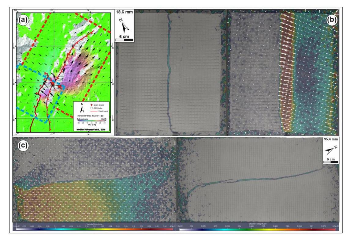
(a) InSAR of 2014 Kamishiro Earthquake. (b) PIV analysis of reverse fault sandbox model. (c) PIV analysis of strike slip fault sandbox model. We overlaid the InSAR model with blue and red dashed box as a reference to the reverse fault and strike slip models, respectively.
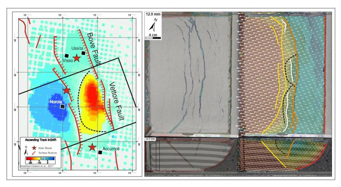
InSAR of the 2016 Central Italy Earthquake (left). PIV of normal fault sandbox experiment (right). We flipped the image to help comparison of both images. We also highlighted several involved faults, which we colored to correspond to Figure 9. Note that the horizontal displacement vector distribution above the normal fault's hanging wall of both images (black dashed line) shows surface movement constrained by fault surface rupture.
Potential Future Studies
Future research stemming from this study could enhance our comprehension of earthquake processes and refine mitigation efforts. This may involve:
- 1. Geological Realism: Researchers can explore a more realistic geological spectrum by employing materials arranged in accordance with the stratigraphy of the study area. Additionally, considering the shape of the indenter and the basement underlying the model as well as the distribution of layer thickness would bring the experimental conditions closer to real-world scenarios.
- 2. Advanced Mapping Technologies: Integration of advanced mapping technologies and techniques, such as high-resolution mapping and laser interferometry methods, could be employed to capture the vertical evolution of the topography. This approach aims to align the sandbox modeling results more closely with InSAR observations, offering a more nuanced understanding of fault behavior and surface deformation.
- 3. Interdisciplinary Collaboration: Facilitating collaboration among geologists, seismologists, and civil engineers can contribute to a comprehensive understanding of earthquake processes. This interdisciplinary approach has the potential to enhance the robustness of earthquake hazard assessments by leveraging diverse expertise and perspectives.
Implementing these suggestions in future research endeavors would not only deepen our understanding of earthquake dynamics but also contribute to more effective strategies for mitigating seismic risks.
Conclusion
This study investigated the relationship between fault kinematics and surficial movement patterns during earthquakes through a combination of InSAR observations and analogue sandbox modeling. The research highlighted the potential of sandbox experiments in simulating various fault systems, providing valuable insight into fault surface rupture development patterns. By comparing these experimental results with InSAR data, we hoped to contribute to the understanding of the complex interplay between fault behavior and surface deformation. The findings emphasize the importance of refining analogue models, incorporating realistic geological features, and leveraging advanced imaging techniques for more accurate seismic hazard assessments.
The detailed analysis of different fault systems – reverse, normal, and strike-slip – highlighted the unique propagation characteristics of each type. These findings challenge existing assumptions in seismic science and call for a more nuanced understanding of fault dynamics. Particularly, this study underscores the importance of considering the role of rock rheology and the distribution of crystalline rocks beneath the surface in predicting fault surface ruptures.
This research lays the groundwork for future studies to delve deeper into the temporal dynamics of fault systems, validate model predictions against real-world seismic events, and foster interdisciplinary collaboration for a comprehensive understanding of earthquake processes. Ultimately, this work aimed to enhance our ability to predict and mitigate the impact of earthquakes on areas where fault surface rupture has not been mapped adequately.