
Introduction
An optimal schedule of hydrothermal power systems (HTPSs) determines the power generation of both thermal power plants (TMPs) and hydroelectric power plants (HDPs) that need to meet load demand at every subperiod in the entire scheduled operation [1-3]. Alongside that, the minimization of the total electricity production expenditure (TEPE) of TMP is also considered. At the same time, the TEPE of HDPs can be abandoned because the operation of these HDPs uses water from rivers that is almost free [4, 5]. Depending on the time length, the optimal scheduling problem (OS) is separated into three categories: short-term [6-12], medium-term [13, 14], and long-term [15, 16]. Recently, the consideration of the short term is more popular than the two others. Specifically, in short-term problems with a fixed head model, the power generation of HDP is modeled by the released function, as published in [10-11]. As varying head models are taken into account, a hydro generation function with respect to reservoir volume and discharge is used [17-20]. Clearly, the hydrothermal system scheduling problem is very important for power systems, and this topic has been widely discussed so far. However, the energy storage in the system is not highly significant due to the characteristics of hydropower plants. Thus, this study considered special hydroelectric power plants, called pumped storage hydroelectric power plants (PSHDPs) as an effective solution to reach the minimum TEPE.
Copyright ©2024 Published by IRCS - ITB J. Eng. Technol. Sci. Vol. 56, No. 1, 2024, 81-94 ISSN: 2337-5779 DOI: 10.5614/j.eng.technol.sci.2024.56.1.7
The basic notion of a typical HTPS includes one TMP and one HDP, in which the generating mode is the sole operation mode. However, in the modified version, the pumped storage hydroelectric power plant (PSHDP) is introduced with two operation modes, i.e., a generating mode and a pumping mode. The main idea of using a PSHDP is to minimize the TEPE of a TMP during several periods in the schedule. This means that at peak load demand periods, the TMP must increase its power generation, increasing the TEPE. In these circumstances, the PSHDP releases water from the reservoir through the hydro turbines to generate electricity and decrease the pressure on the TMP. In contrast, when load demand is low, the abandoned power is used to run the pumping mode in the PSHDP to pump water back to the reservoir.
The study reported in [21] was one of the first to evaluate the contribution of the PSHDP to the HTPS. Specifically, the study proposed the former notion of a HTPS with one HDP, one PSHDP, and one TMD. Then, the authors applied the gradient method to find the best generation schedule for all plants. The key contribution of the study was to indicate that the applied method can satisfy all the related constraints of these power plants, especially the constraints of a PSHDP.
In [22], the authors introduced another method to solve the OS problem, called two-phase computation (TCP), to assist in the selection between generating mode and pumping mode. According to the results reported by the authors, TCP proved to be an effective method to deal with the problem, with the main objective function of reducing the TEPE of the TMP over 24 hours. However, the specification of the applied system was not clearly shown.
The methods mentioned in [21, 22] are classical computing methods, which have several shortcomings: a slow response, requiring many complex calculations, being unable to reach the optimal solution, being unable to deal with all constraints of large systems with a high number of control variables, etc. Being aware of the weaknesses of the classical methods, researchers have applied meta-heuristic methods with several advantages, such as ease of application, a quick response, not requiring much computation, and feasible to reach optimal solutions for problems with a large search space. The application of the meta-heuristic algorithms can be divided into two groups. In the first group, the authors applied the original version of the algorithm, while the researchers in the second group applied the algorithms with different modifications to the update mechanism to improve the efficiency of the modified algorithm over the original one.
Typical applications of the improved version of the original meta-heuristic algorithms can be found in studies [23-25]. Specifically, in [23], static and dynamic parameters were added to enhance the efficiency of PSO's search process. In [24, 25], the authors added three random factors in the position update model of the accelerated particle swarm optimization (APSO) to boost the ability to reach the global solution. In [26], the authors also proposed an improved version of the differential evolution algorithm (DE), called the Phase-Based Adaptive Differential Evolution algorithm (PBA-DE). Meanwhile, the application of the original version of the meta-heuristic methods is also very popular. This implementation can be found in studies [27, 28], using evolutionary programming (EP).
Most of the above-mentioned studies commonly focus on determining optimization generation for the HTPS operation over a short-term period by using meta-heuristic algorithms. However, several shortcomings need to be addressed:
- 1. The efficiency of the improved method over the original version has not been clarified in detail. For example, in [25], the author proposed the AFPSO to solve the optimization generation for the HTPS, but application of the original method was not executed for comparison with the proposed method.
- 2. The results reported in [12] and [27] only focused on shortening the TEPE of the TMP rather than strictly respecting the related constraints of the given problem.
- 3. Integration of renewable energy sources such as wind and solar energy was not the first priority.
- 4. The revenue obtained by operating the HTPS following the optimal schedule found by the applied method was not evaluated.
By acknowledging all these shortcomings from the previous studies, as mentioned above, this research was conducted to fully solve the optimization generation problem for HTPS and remove all flaws found previously. Specifically, the Self-Organizing Migration Optimization (SOMA) algorithm [29] and its improved version (ISOMA)
were applied to solve the problem with two main objective functions, i.e., minimizing the TEPE of the TMP and maximizing the total profit for operating the HTPS. Besides, the contribution of renewable energy sources such as wind and solar was also taken into account while reaching the second objective function. According to [29], the earliest version of SOMA, proposed in the 2000s, was based on swarm intelligence. Particularly, the whole searching process for the optimal solution of SOMA imitates the competition and cooperation practices of the individuals in a particular population through many of migrating loops. By acknowledging the strengths and weaknesses of the early version of the SOMA, ISOMA was proposed with a key improvement on the update mechanism for better efficiency over the early version. The main contributions of the whole study can be recapped as follows:
- 1. Successfully propose an improved version of SOMA (ISOMA) to solve the HTPS problem for a period of 24 hours
- 2. Indicate the improvement of ISOMA over its early version and other state-of-the-art meta-heuristic algorithms in terms of the TEPE value of the TMP in a period of 24 hours in the first system.
- 3. ISOMA successfully considers both wind and solar energy and reaches more profit than SOMA in the second system.
- 4. Diversify the trend of improving the former meta-heuristic algorithms to achieve better performance.
The Problem Description
The Main Objective Functions
The present study applied ISOMA for two study cases with different objective functions. In the first case, ISOMA solved an existing system with one thermal power plant (THP) and one storage hydroelectric power plant (PSHDP) to reach the minimum total electricity production expenditure (TEPE). In the second case, ISOMA solved an expanded system by integrating one wind and one solar power plant into the existing system to maximize the total profit (TPRF). The two objective functions were formulated as follows:
The First Objective Function
The operation of TMPs expends a generation cost, called the total electricity production expenditure (TEPE), where the TEPE must be reduced as much as possible. Generally, TEPE is expressed by a square function, as considered in [26]. In addition, while the TEPE is considered in the hydrothermal scheduling problem (HTS), short-term hydrothermal scheduling is also considered. The determination of the TEPE was modified as mentioned in [28], which is given as in Eq. (1):
Minimize \[TEPE = \sum_{s=1}^{SI} \sum_{k=1}^{n_1} (\alpha_{1k} + \alpha_{2k} PTM_{k,s} + \alpha_{3k} PTM_{k,s}^2)\] (1)
where SI is the number of subperiods in the given schedule (it was selected to be 24 hours for a day in this study); \(n_1\) is the number of thermal power plants (TMPs); \(\alpha_{1k}\), \(\alpha_{2k}\) and \(\alpha_{3k}\) are the known coefficients of the TMP k with \(k = 1, 2, ..., n_1\); and \(PTM_{k,s}\) is the power generated by the TMP k in subperiod s.
The Second Objective Function
The second objective function was used to maximize the total profit while operating the HTPS. The mathematical expression of this objective function was formulated as follows:
\[Maximize\ TPRF = \sum_{s=1}^{SI} (ReVe_s - TEPE_s)\] (2)
\[ReVe = \sum_{s=1}^{SI} (PRC_s \times PDM_s)\] (3)
In Eqs. (2) and (3), TPRF is the total profit; \(ReVe_s\) is the revenue obtained in subperiod s; \(PRC_s\) is the price of the electricity sold to customers in subperiod s, and was known as a given data before implementing the optimization operation for the hybrid system in the second study case; and \(PDM_s\) is the power demand in subperiod s.
The Related Constraints
Power balance constraint of the generating and consuming sides: this constraint means that the total power produced by all generating sources must be equal to the power required by the consuming side (PDM) plus power loss (PLS) in the transmission lines. In [12], the mathematical expression of this constraint is described as follows:
\[\sum_{k=1}^{n_1} PTM_{k,s} + \sum_{m=1}^{n_2} (S_{m,s}.PTH_{m,s}) - \sum_{m=1}^{n_2} [(1 - S_{m,s})PSH_{m,s}] - PDM_s - PLS_s = 0\] (4)
where \(n_2\) is the number of pumped storage hydroelectric power plants; \(PTH_{m,s}\) is the power output produced by the PSHDP m in subperiod s; \(PSH_{m,s}\) is the pump power of the PSHDP m in subperiod s; \(S_{m,s}\) is the operating mode of the m-th PSHDP in the s-th subinterval. In each operating subperiod, the m-th PSHDP can have one out of three modes, i.e., generating, pumping, and off. \(S_{m,s}\) is set to 1 when the operating mode is generating. \(S_{m,s}\) is set to 0 when the operating mode is pumping. When the operating mode is pumping, the pump power \(PSH_{m,s}\) is set to the maximum generation limit; meanwhile, the generation power is 0 MW. When the operating mode is off, the generation and the pumping power are 0 MW. The operating modes \(S_{m,s}\), pumping power \(PSH_{m,s}\), and generation power \(PTH_{m,s}\) are summarized as follows in Eq. (5):
Operating mode = \[\begin{cases} generating, then \ S_{m,s} = 1, PTH_{m,s} > 0 \ and \ PSH_{m,s} = 0 \\ off, & then \ PTH_{m,s} = 0 \ and \ PSH_{m,s} = 0 \\ Pumping, \ then \ S_{m,s} = 0, PTH_{m,s} = 0 \ and \ PSH_{m,s} = PTH_m^{max} \end{cases}\] (5)
Here, \(PTH_m^{max}\) is the maximum generation limit of the m-th PSHDP.
Constraint about the amount of released water from the reservoir: this constraint is mentioned in [9]. The study indicated how much water was ready to be released to the hydro turbine for producing electricity:
\[WRS_{m.s} = TL_s \times PW_{m.s} \tag{6}\] where \(WRS_{m,s}\) is the amount of released water streaming down to the hydro turbine of \(HDP\ m\) in subperiod s; \(TL_s\) is the length of subperiod s; and \(PW_{m,s}\) is the proportion of released water of \(HDP\ m\) in subperiod s. In [9], \(PW_{m,s}\) is obtained by applying in Eq. (7):
\[PW_{m,s} = \beta_{1m} + \beta_{2m}PTH_{m,s} + \beta_{3m}PTH_{m,s}^2\] (7)
where \(\beta_{1m}\), \(\beta_{2m}\) and \(\beta_{3m}\) are coefficients of the released water proportion over the produced power output of PSHDP m.
Constraint of balance of water in reservoir: In [9], this constraint is the relationship among three elements, i.e., the inflow, the released, and the pumped water. These elements are bound by the following constraint in Eq. (8):
\[WSS_{m,s-1} - WSS_{m,s} + WSB_{m,s} - WRS_{m,s} + WSI_{m,s} = 0\] (8)
where \(WSS_{m,s-1}\) and \(WSS_{m,s}\) are the amounts of water available inside the reservoir m in subperiods s-1 and s; \(WSB_{m,s}\) is the amount of water going back to the upper reservoir during the pumping mode of PSHDP m in subperiod s; and \(WSI_{m,s}\) is the volume of water inflow to the reservoir of PSHDP m in subperiod s.
Constraint of water level at the initial point and the final point: According to [23], the water stored in reservoir must be restricted as follows:
\[WSS_{m,0} = WSS_{m,ini}; WSS_{m,SI} = WSS_{m,fin}\] (9)
where \(WSS_{m,ini}\) and \(WSS_{m,fin}\) are the water levels in the reservoir of PSHDP m at the initial point and the final point of the schedule; \(WSS_{m,SI}\) are the water levels in the reservoir of PSHDP m before it is optimized and during the last subperiod SI.
Constraint of water allowed to be stored in the reservoir: For safety reason as mentioned in [12], the capacity of storing water in the reservoir must be located within safe boundaries as described in the mathematical model below:
\[WSS_m^{min} \le WSS_m \le WSS_m^{max} \tag{10}\] where \(WSS_m^{min}\) and \(WSS_m^{max}\) are the lowest and the highest level of the water stored in the reservoir of the PSHDP.
Constraint of water released: This constraint is about the proportion of the water released to the hydro turbines. In [27], this constraint is formulated as follows:
\[PW_m^{min} \le PW_{m.s} \le PW_m^{max} = 1, 2, ..., n_2; s=1, 2, ..., SI\] (11)
where \(PW_m^{min}\) and \(PW_m^{max}\) are the lowest and the highest proportion of released water from the upper reservoir of PSHDP m.
Operation constraint of the generating mode and the pumping mode: This constraint is about the physical limits in the operation of both the TMP and the HDP. This means that the amount of power output produced by these power plants must be located within allowed ranges. Besides, the power utilized for the pumping mode of the PSHDP is also restricted in predetermined range. In [12], the mentioned ranges were formulated as follows:
\[TMP_n^{min} \le TMP_{n.s} \le TMP_n^{max} \tag{12}\]
\[PTH_m^{min} \le PTH_m \le PTH_m^{max} \tag{13}\]
\[PSH_m^{min} \le PSH_m \le PSH_m^{max} \tag{14}\]
In Eqs. (12) to (14), \(TMP_n^{min}\) and \(TMP_n^{max}\) are the lowest and highest value of the power output produced by TMP n; \(TMP_{n,s}\) is the power output produced by TMP n in subperiod s; \(PTH_m^{min}\) is the lowest power output of the PSHDP; \(PSH_m^{min}\) and \(PSH_m^{max}\) are the lowest and the highest power utilized by PSHDP m; and \(PSH_{m,s}\) is the power utilized by PSHDP m in subperiod s.
Searching Methods
Original Self-Organizing Migrating Algorithm (SOMA)
Like other metaheuristic algorithms such as particle swarm optimization, cuckoo search, differential evolution, and so on, the structure of the SOMA also comprises of three main stages, consisting of finding new solutions, calculating the fitness function, and keeping promising solutions. Basically, almost all metaheuristic algorithms use the same fitness function calculation and the same selection of promising solutions but different structures of new solution generation techniques. In this section, a new solution update procedure of SOMA is presented, and then the procedure is modified in the next section.
The update process for new solutions of the original SOMA is executed by using the following mathematical expression:
\[S_p^{MR+1} = S_p^{MR} + \left(S_{LD}^{MR} - S_p^{MR}\right) \times k \times CRT \times VR \text{ with } p = 1, 2, \dots, PZ - NL\] (15)
Where \(S_p^{MR+1}\) is the new position of individual p in loop (MR+1); \(S_{LD}^{MR}\) is the position of the leader individual in the current loop, MR; \(S_p^{MR}\) is the current position of individual p; k is the moving factor; CRT is the chaotic factor; VR is the vectoring regulator; PZ is the value of the initial population; and NL is the number of leaders in each loop. There are three parameters, k, VR, and CRT, which are determined by:
\[k = (N_{SL} - n_i + 1) \times SL \text{ with } i = 1, ... N_{SL}\] (16)
\[VR = \begin{cases} 1, & if \ RnD < CRT \\ 0, & otherwise \end{cases}\] (17)
\[CRT = 0.1 + 0.9 \times \left(\frac{EVL}{FVL^{max}}\right) \tag{18}\]
In Eq. (16), \(N_{SL}\) is the number of jumping steps; \(n_i\) is the jumping step size, i; and SL is the length of each jumping step. In Eq. (17), RnD is a randomized value between 1 and 0. In Eq. (18), EVL and \(EVL^{max}\) are the number of fitness evaluations and the maximum fitness evaluation number.
The Modified Self-Organizing Migrating Algorithm (ISOMA)
As shown in Eqs. (15) and (17), the update procedure of SOMA is much dependent on randomization factor VR. As pointed out in Eq. (17), VR has two different values, either 1 or 0. If VR is equal to 0, the second term on the right-hand side of Eq. (15) is equal to 0. As a result, the new solution \(S_p^{MR+1}\) and the old solution \(S_p^{MR}\) are the same. This means that the p-th solution is not newly updated. As the random number RnD in Eq. (17) is smaller than CRT obtained by using Eq. (18), VR will get a value of 0. To see the impact of CRT on the update procedure of SOMA, CRT and VR were simulated over 100 iterations with the selection of 20 for the population. The simulation results are reported in Figure 1. The figure indicates that CRT increased linearly as the iteration increased. Random number RnD changed within 0 and 1, whereas VR had two values, 0 or 1. Clearly, for cases where RnD is higher than CRT, and VR gets zero values. For other cases where RnD is not greater than CRT, VR becomes 1. VR got many 0 values over 100 iterations. This means that there were many iterations where the new solution \(S_p^{MR+1}\) was the same as the old solution \(S_p^{MR}\). The effectiveness of SOMA is restricted due to the case of VR = 0. Hence, Eq. (15) was modified as in Eq. (19).
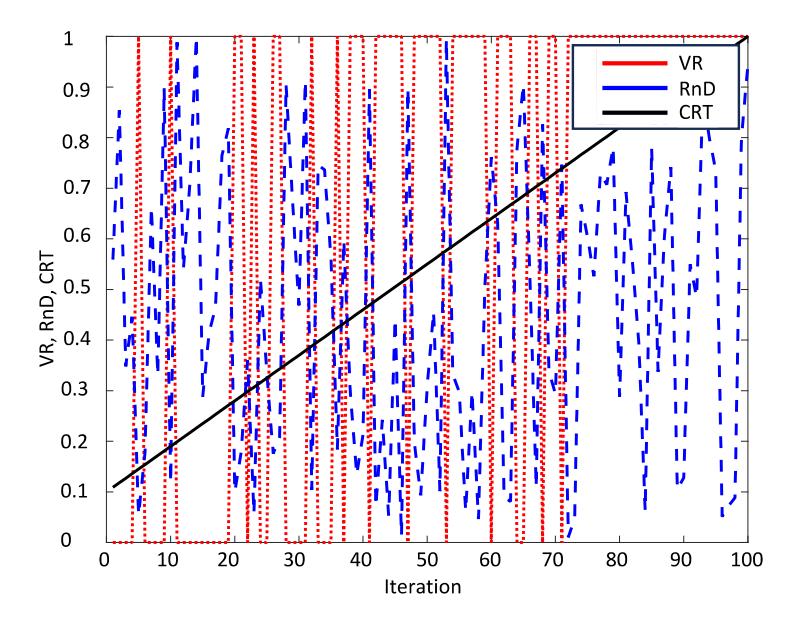
Figure 1Simulation result of CRT and VR over 100 computation iterations.
\[S_p^{MR+1} = S_p^{MR} + \left(S_{LD}^{MR} - S_p^{MR}\right) \times k \times CRT \times VR \times srf_1\] \[+ \left(S_{LD}^{MR} - S_p^{MR}\right) \times RnD \times srf_2 ; with p = 1, 2, ..., PZ - NL\] (19)
In the formula, \(srf_1\) and \(srf_2\) are the shrinking factors, which are selected randomly in a range from 0.1 to 0.5. The use of \(srf_1\) in the first jumping step is done to narrow the size of the first step; meanwhile, the second step is very important to enlarge the searching zone for the last computation iterations. The combination is very useful in finding more appropriate zones for reaching good solutions. The proposed modification is the key factor in achieving better results with ISOMA, while SOMA cannot reach the same best solution and the same performance for the problem considered in this paper.
Results and Discussions
In this section, both SOMA and ISOMA will be applied to determine the optimization generation of HTPS in two different case studies. The description of each case study is as follows:
- 1. Case 1: The first objective function, minimizing the total generation cost of the thermal power plant, shown in Eq. (1), was applied for the first HTPS. The HTPS comprised one TMP and one PSHDP without renewable energies (RESs). In Case 1, we compared the total generation cost (TEPE) of ISOMA with that of SOMA and other algorithms, namely EP in [27], AFPSO in [25], and APSO in [24]. The comparison was aimed at seeing if ISOMA was more effective than the other algorithms and would be more suitable for the simulation in Case 2.
- 2. Case 2: The second objective function, maximizing the total profit, shown in Eq. (2), was applied for the second HTPS. The second HTPS was an expanded system that integrated one solar and one wind power plant into the first system from Case 1. In Case 2, we compared ISOMA's total profit with that of SOMA. As a result, we found that ISOMA could reach a greater total profit than SOMA. Thus, ISOMA effectively maximized the total profit of the hybrid power system with one TMP, one PSHDP, one solar power plant, and one wind power plant.
To further highlight the improvement of ISOMA over SOMA, these methods were set with the same control parameters in terms of the path length, step, maximum number of iterations, maximum number of fitness evaluations, and number of independent runs. These settings were 3.0, 0.11, 1000, 50000, and 50, respectively.
All the related work for this study was executed on a personal computer with the following basic specifications: central processing unit (CPU) Intel Core i7-12700H with 2.6 GHz of clock speed, random access memory (RAM) DDR5 8GB with bandwidth 4800 Gb/s. All codes and simulations were compiled in the Matlab program, version 2018b.
Results Achieved in Case Study 1
The case study was performed on a system with one TMP and one PSHDP over 24 hours. The power system configuration and the load demand within 24 hours are described in Figures 2 and 3. Note that the power losses on lines were ignored.
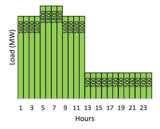
Figure 2 The power system illustration.
Figure 3 Load demand within 24 hours.
Figure 4 shows the summary after 50 independent runs of both SOMA and ISOMA. The black curve stands for the results obtained by SOMA, while the red one represents the same values achieved by ISOMA. By observing the figure, the proposed ISOMA could achieve more optimal results than SOMA during 50 independent runs. The results mean that ISOMA showed superiority over SOMA while dealing with the optimization generation problem with the objective function of minimizing the TEPE of the TMP.
The superiority of ISOMA over SOMA is shown further in Figure 5. In the figure, the results obtained by the two applied methods are compared in terms of the minimum TEPE, mean TEPE, and maximum TEPE. ISOMA completely outperformed SOMA on all criteria. Specifically, while the minimum TEPE achieved by ISOMA was only 269,216.8 ($), the same value reported by SOMA was up to 269,644.1($). The cost savings for the TEPE on this criterion was 427.3($), or 0.16%. While observing the mean TEPE and the maximum TEPE, the values
achieved by ISOMA were all better than those achieved by SOMA. Particularly, the results achieved by ISOMA on these criteria were 269,623.0($) and 269,655.3($), respectively, while similar results given by SOMA were 269,649.8($) for the mean TEPE and up to 269,682.0($) for the maximum TEPE. The cost savings of ISOMA over SOMA for the mean TEPE and max TEPE were 26.8($) and 26.7($), respectively.
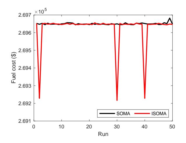
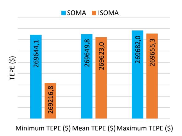
Figure 4 The results achieved by both SOMA and ISOMA after 50 independent runs.
Figure 5 Comparison between SOMA and ISOMA on different criteria.
In Figure 6, the minimum TEPE achieved by ISOMA is compared with the results obtained by other methods, such as EP in [27], AFPSO in [25], and APSO in [24]. In the figure, it is easy to recognize that the TEPE value obtained by ISOMA was overall better than that of the other methods. The cost savings in percentage of ISOMA over EP, AFPSO, and APSO was 0.16%.
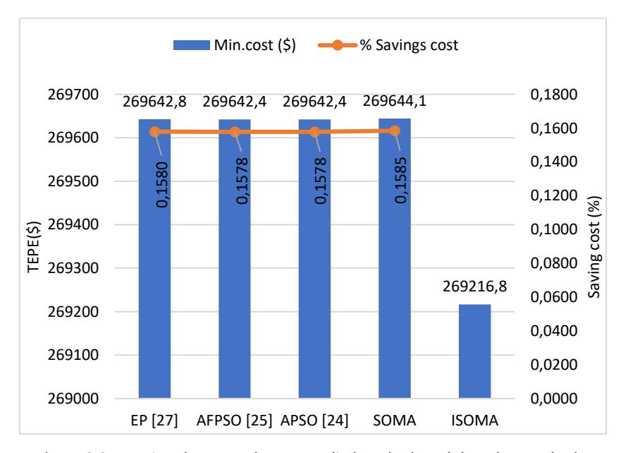
Figure 6 Comparison between the two applied methods and the other methods.
Figure 7 shows the water level in the reservoir of the PSHDP within 24 hours found by ISOMA. In the figure, ISOMA satisfies all the related constraints of the hydropower plant. Specifically, the water level at the initial point and the final point of the whole schedule are equal. The amount of water storage represented by the red line varied within the allowed ranges. Also, the volume of released water satisfied its constraint.
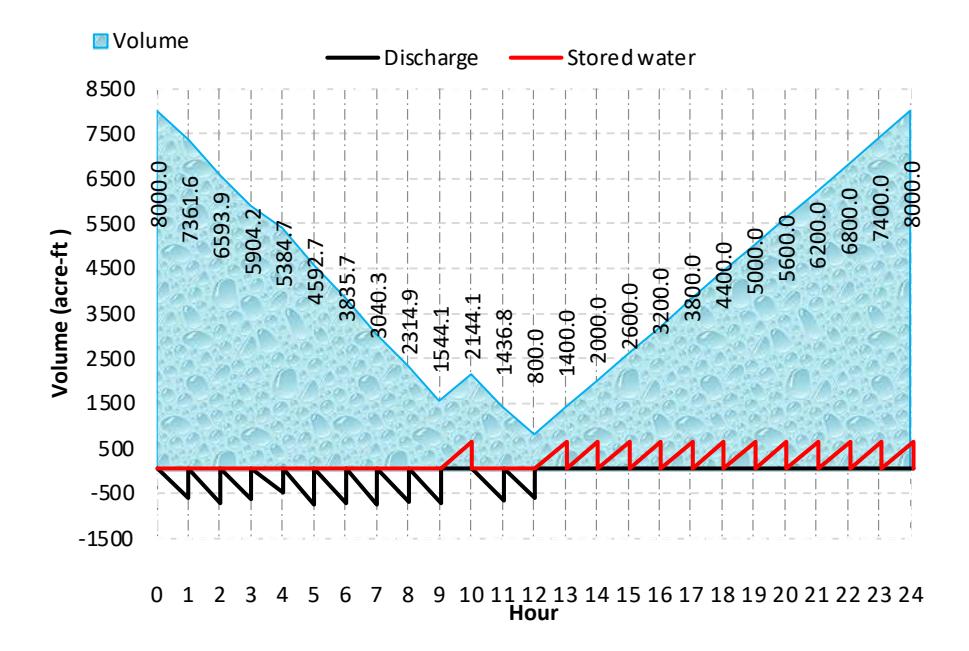
Figure 7 Reservoir volume of the PSHDP in Case Study 1 for 24 hours.
The Results Achieved in Case Study 2
In this section, both the wind and solar generators were connected to the first power system, as described in Figure 8. The related data about the power output of wind power plants (Windpower), the power output of solar power plants (PV power), and the electricity price for each hour were taken from [30], [31], and [32], respectively. These data are presented again in Figure 9. Recall that the main objective function in this case study was used to maximize the total profit (TPRF) of operating the HTPS.
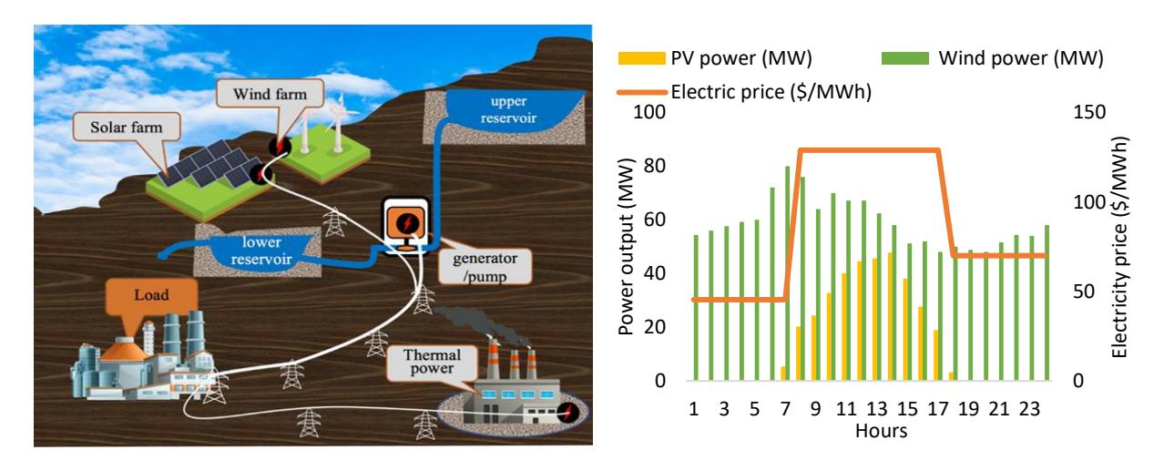
Figure 8 Power system used in Case Study 2 with the presences of both wind and solar energy.
Figure 9 The power output of the wind and solar generators, and the electricity price.
Figure 10 shows that the application of ISOMA increases the TPRF values over SOMA in terms of the maximum profit, mean profit, and minimum profit. Specifically, the additional profit brought by ISOMA over SOMA at the maximum TPRF was 0.4 ($), while the same values in terms of mean TPRF and minimum TPFR were 2.5 ($) and 5.3 ($), respectively.
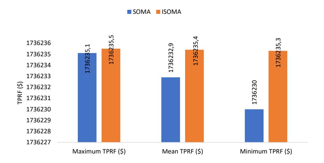
Figure 10 The profit obtained by both SOMA and ISOMA with the second objective function.
Figure 11 shows the reservoir volume of the PSHDP within 24 hours found by SOMA. By observing the figure, all related constraints, such as the constraint of the water level at the initial and final points, the constraint of allowed water stored in the reservoir, and the constraint of released water, are all satisfied.
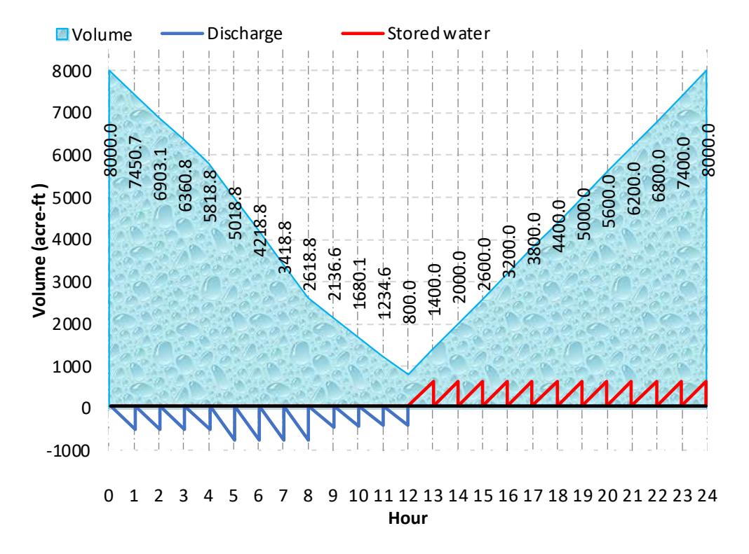
Figure 11 Water volume in the reservoir of the PSHDP in Case Study 2 during 24 hours.
Volume, inflow, stored water, and discharge of PSHDP for the two cases in the most effective solution reached by ISOMA are presented in Table A1 and Table A2 in the Appendix.
Conclusion
This study proposed a successfully improved version of the self-organizing migration algorithm (ISOMA) to determine the optimization generation for an HTPS. The efficiency of the new method was validated in different case studies, including Case 1, with the main objective function minimizing the TEPE of the thermal power plant, and Case 2, with the main objective function maximizing the TPRF of the HTPS operation. Besides, both wind and solar energy were taken into account in the power system used in Case 2. The results obtained in Case 1 indicate that ISOMA completely outperformed SOMA on all compared criteria. Specifically, ISOMA saved 427.3 ($) or 0.16% of the TEPE value over SOMA. Besides, when ISOMA was compared with other methods (EP, AFPSO, and APSO), the efficiency percentage of ISOMA compared to these methods was approximately 0.16% better in each case. The evaluation of the results obtained in Case 2 also points out that ISOMA is completely superior to SOMA in terms of maximum TPRF, mean TPRF, and minimum TPRF. As a result, ISOMA can be considered an efficient search method. Therefore, we suggest using ISOMA to deal with the optimization generation problem of HTPS.
Regardless of the positive results obtained by ISOMA, there are also some shortcomings that need to be improved in this study. For example, the scale of the power system is very small and impractical in practice; features of the electricity market were not clearly considered; the improvement of ISOMA over SOMA and other compared methods were not significant enough for a breakthrough; ISOMA focused on modifying the updating mechanism, while other auxiliary parameters that heavily affect the whole searching process remained the same. In the future, the optimization generation problem for HTPS should be solved on a larger scale, and the rules of the electricity market should be deeply evaluated. SOMA should be improved more to reach a higher degree of efficiency for dealing with a larger scale of the optimization generation problem for HTPS. Furthermore, optimization software to solve problems in power systems, such as ETAP, Powerworld, Power system optimizer, and Gurobi optimizer, will be applied for result comparisons with proposed versions of SOMA. Among this software, Gurobi optimizer is a promising optimization tool for complex nonlinear problems. It can reach global optimal solutions of complex nonlinear problems at high speed. The development of effective metaheuristic algorithms and the use of high-performance software, in addition to the consideration of largescale and real power systems, are expected to result in significantly valuable future studies.
Acknowledgement
This research is funded by Foundation for Science and Technology Development of Ton Duc Thang University (FOSTECT), website: http://fostect.tdtu.edu.vn, under Grant FOSTECT.2023.34.