
Introduction
Unmanned aerial vehicles (UAVs) are widely used in various applications nowadays, such as military, coastal guard, survey, agriculture, etc. [1, 2], since UAVs do not require a human pilot on board. This is advantageous for most flight missions, particularly for dangerous missions [3]. The design of a UAV concerns several aspects such as maximizing flight performance, minimizing energy consumption, etc. [4-6]. For the energy consumption aspect, design optimization of the propeller is an interesting topic to improve UAV performance, while the objective functions considered are for example maximizing power output or thrust [7-9], etc. [10, 11]. The design variables considered were for example blade pitch, chord length, thickness, blade span, number of blades, blade angle of attack, and airfoil profiles [9-12].
The optimum design of a propeller or other engineering problems are usually based on metaheuristic optimizers (MHOs) since the objective functions and constraints imposed are usually evaluated by means of numerical simulation to which, sometimes, conventional gradient-based optimizers may not be suitably applied due to the difficulty of function gradient approximation. Compared to gradient-based optimizers, MHOs have some advantages, such as no requirement of function derivatives, global optimization, and being able to explore a Pareto front within a single run for the case of multi-objective optimization. As a result, they can deal with almost any kind of function and design variable. Some of the various kinds of function and design variables are: engineering economics optimization [13], heat exchanger design [14-16], sterling engine and fuel cell hybrid optimization [17, 18], an automobile suspension arm [19], etc. However, it is well known that MHOs have some disadvantages, such as slow convergence rate and inconsistency. Consequently, performing optimization using
Copyright ©2024 Published by IRCS - ITB J. Eng. Technol. Sci. Vol. 56, No. 3, 2024, 404-413
MHOs usually requires numerous function evaluations. Therefore, the optimum design of a propeller or other engineering problems are mostly carried out based on low-fidelity simulation such as blade element momentum theory (BEM) [11] or a vortex lattice method (VLM) [20, 21], while the implemented MHOs include a genetic algorithm (GA) [11], particle swarm optimization (PSO) [22], differential evolution (DE) [23], etc.
Recently, high-fidelity computation such as computational fluid dynamics (CFD) has become a popular tool in the field of fluid flow analysis [1,24-27], which also includes propeller design [28-32], as it is more accurate and more suitable for various simulation conditions than BEM and VLM. Moreover, it is known to produce results that are as accurate as those from wind tunnel testing [33, 34]. However, due to its expensive computation requirements, it is almost impossible to perform MH optimization based on the CFD directly. The use of surrogate-assisted MHOs is a solution for such problems. The main idea of using surrogate-assisted MHOs is that a high-fidelity simulation based on CFD is performed for some training points in the design domain, while the points are generated by means of design of experiment (DoE). Then, a surrogate model is constructed based on the design training points, which is used for function approximation while performing optimization is done using MHOs. After the optimum points are obtained, their actual function values are evaluated using a high-fidelity simulation. This technique can reduce computational cost and has been successfully applied in various optimization problems. For propeller optimization, several surrogate models have been applied, e.g., response surface model (RSM) [35], radial basis function model (RBF) [36], Kriging model (KG) [37], etc. [38], while the used MHOs are mostly based on classical algorithms such as GA [37, 39], DE [28], or PSO [22]. Arguably the most used DoE is the Latin hypercube sampling (LHS) technique. In fact, the quality of the optimum solution obtained from using surrogate-assisted MHOs depends on three main factors: the surrogate model technique, the MH algorithm, and the DoE technique. Among several surrogate model techniques, KG is one of the most popular methods due to its superiority in prediction accuracy [37, 40, 41]. However, performance investigation of using a KG surrogate model with several MH techniques for optimization of UAV propellers was not found in the literature. In addition, applying an optimum Latin hypercube sampling technique (OLHS), which has been found to have better space filling in the design domain than the original LHS, has rarely been done for such a design problem.
Therefore, this work presents a propeller design for an UAV using a KG surrogate model, while seven MH algorithms were implemented. The design problem was posed to maximize the propeller efficiency while the design variables were the twist angle and the ratio of blade thickness to chord length of a twenty airfoil sections. CFD analysis was used for high-fidelity aerodynamics simulation of the propeller. The KG surrogate model was used as the surrogate model, while an OLHS proposed by Pholdee and Bureerat in [42] was used as the DoE technique. Several MH optimizers, including GA [43], PSO [44], population-based incremental learning (PBIL) [45], DE [46], teaching-learning based optimization (TLBO) [47], ant colony optimization (ACO) [48], and an evolution strategy with covariance matrix adaptation (CMA-ES) [49], were used to solve the proposed problem and their performances were investigated.
Formulation for Optimization Problem
Optimization Problem
In this work, the design problem proposed was the optimization of a two-blade propeller for an UAV at a motor speed of 6,500 rpm. The design problem was posed to maximize the propeller efficiency while the design variables were the twist angles and the ratio of blade thickness to chord length of twenty airfoil sections. To maximize the propeller efficiency, an objective function can be expressed by minimizing ratio of thrust to torque as follows:
\[f(x) \left[ \frac{T - T_{max}}{Q - Q_{min}} \right]_{min} \tag{1}\]
subjected to −12.5% ≤ ≤ 12.5%, 0.12 ≤ ≤ 0.13 where = {, } is a set of design parameters including the twist angles and the ratio of propeller thickness to chord length, respectively. and are the thrust and the rotation torque, respectively. and are the maximum thrust and the minimum torque obtained from DoE. It should be noted that the twist angles and chord
length were used to form the propeller profile of APC Thin Electric 9×6 [50] to modify the design value. While the maximal relative thickness of the propeller was extended to cover the bound from the study of Kovačević [39].
Aerodynamics Analysis of Propeller
To analyse the propeller aerodynamics, the CFD code under the commercial software ANSYS/Fluent was used. As illustrated in Figure 1, the CFD model was defined by a stationary domain of a 10D cube, while the rotating domain wasset to 1.1D dimeter, where D represents a propeller diameter of 228.6 mm. Here, the CFD simulation created a sufficiently enlarged domain to reduce the turbulent flow influence of air around the rotating propeller. The fluid properties used an air density and a viscosity of 1.225 kg/m3 and 1.7894x10⁻⁵ kg/m-s, respectively, while Reynolds-averaged Navier–Stokes (RANS) with the Realizable − turbulence model was used for steady state flow simulation. The simulation domains consisted of the two domains between the stationary domain and the rotating domain with a moving reference frame of 6500 rpm, while the connection of both domains used the mesh interface option.
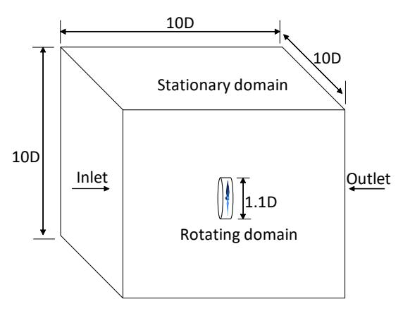
CFD domain analysis.
The boundary conditions were defined at the inlet wall and outlet wall as outflow. The propeller was assigned as a moving wall and the other wall as a stationary wall. The coupled scheme algorithm was used to solve the velocity-pressure coupling in the numerical analysis. The second-order upwind technique was applied to set the pressure, momentum, turbulent kinetic energy, and turbulent dissipation rates. The iteration calculation was defined the residual values of 10-5 .
The grid/mesh model was generated based on a tetrahedron construction to fit the propeller shape, while the first layer thickness was defined with a height of 1x10⁻⁵ m and twenty-five layers were defined for the propeller surface as illustrated in Figure 2. The mesh quality validation was performed to compare the results of propeller efficiency, which modified the mesh density on CFD calculations as illustrated in Figure 3. The mesh density is presented ranging from 1.2 to 4.4 million elements to find the minimum uncertainty of the CFD results.
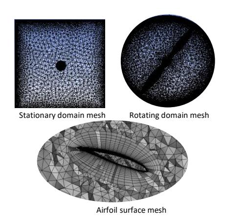
Mesh construction of CFD analysis.
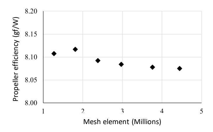
Meshing validation of CFD uncertainty.
In addition, the CFD analysis was verified with the experimental results of thrust, torque, and propeller efficiency, as illustrated in Figure 4-6, respectively. This CFD verification used the propeller model of RCbenchmark × Xoar 9 × 4 and the experimental results from the Tyto Robotics Database [51]. The results between the CFD analysis and the experiment were compared at a propeller speed from 3,849 to 9,333 rpm. The thrust and the torque revealed that the CFD simulation produced slightly higher calculation values than the test results. However, the trends of both the CFD and the experimental results were similar, which means the optimum results from CFD should also agree well with the experimental results. In addition, under the results of thrust and torque as illustrated in Figures 4 and 5, the propeller efficiency was calculated as follows:
\[\eta_p = \frac{T}{Q\omega} \tag{2}\] where is the propeller efficiency and is the rotating speed. The results of propeller efficiency calculated from Eq. (2) are illustrated in Figure 6. The comparison results between the CFD analysis and the experiment of propeller efficiency confirmed that the numerical simulation for rotor aerodynamics was acceptable. The average error was 7.5% for the speed range of 3,849 to 9,333 rpm. Thus, this work used CFD to analyse the aerodynamics of the rotating propeller at 6,500 rpm, i.e., numerical results with error lower than 10%.
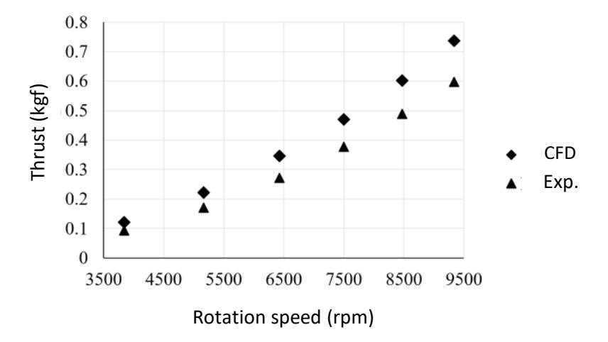
CFD validation with thrust result.
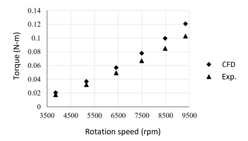
CFD validation with torque result.
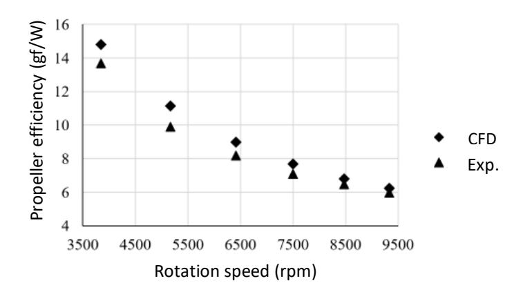
CFD validation with propeller efficiency.
Kriging Surrogate Model-Assisted Optimization
Conventional surrogate-assisted optimization consisted of three main steps i.e., 1) generating a set of sampling points based on DoE and evaluating their real function values; 2) constructing a surrogate model based on the sampling points; 3) performing optimization based on the constructed surrogate model. Finally, the optimum solution obtained was verified again with the real objective function (CFD simulation). In this work, nine sampling points were generated first, based on the OLHS scheme developed by Pholdee and Bureerat in [42]. The CFD was used to verify their objective function values. The KG surrogate model was then constructed based on the set of sampling points. The KG approximation function can be expressed as follows [52]:
\[F(x) = \mu T^{-1} (f - \mu_{min}())_{min}\] (3)
where, () is the predicted function required at a given point , while is the correlation matrix of the sampling points and ; is correlation matrix for all the sampling points, and 1 is a vector full of ones. The variable is expressed as:
\[\mu \frac{{_{1}^{T}}\Psi^{1}f}{{_{1}^{T}}\Psi^{1}1}_{min} \tag{4}\] where is the vector of function values of the sampling points. The KG model used in this study was based the MATLAB toolbox DACE [53], while a Gaussian correlation function was used [54].
Seven well-known MHOs, i.e., GA [43], PSO [44], PBIL [45], DE [46], TLBO [47], ACO [48], and CMA-ES [49], were used to solve the design problem based on the constructed KG model, with five independent runs. After the optimum results were obtained, the CFD was used for their real function evaluation. The results obtained from the various MHOs are discussed below. The overall framework of this study is illustrated in Figure 7.
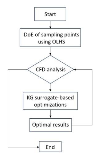
Flow chart of methodology.
Results and Discussion
The results after performing OLHS to generate nine sampling points and evaluating their objective function values based on CFD are reported in Table 1. The minimum and maximum thrusts are given by sampling numbers 3 (Sampling 3) and 1 (Sampling 1), respectively, while the minimum and maximum torques are also given by sampling numbers 3 and 1. It is shown that the set of design variables that gives a lower thrust tends to have a lower torque while, on other hand, the set of design variables that gives a higher thrust lead to a higher torque. Among the 9 sampling points, the maximum propeller efficiency was 9.9915 gf/W, which is given by sampling solution number 3.
| Parameters | DoE | CFD | ||||
|---|---|---|---|---|---|---|
| 𝜽(%) | 𝒕 𝑪 | 𝑻(𝒌𝒈𝒇) | 𝑸(𝑵𝒎) | 𝒈𝒇 𝜼𝒑 ( ) 𝒘 | ||
| Sampling 1 | 11.9222 | 0.1247 | 0.4873 | 0.0886 | 8.0778 | |
| Sampling 2 | -5.5556 | 0.1231 | 0.4444 | 0.0681 | 9.5816 | |
| Sampling 3 | -11.7452 | 0.1237 | 0.4282 | 0.0630 | 9.9915 | |
| Sampling 4 | 8.3333 | 0.1260 | 0.4814 | 0.0853 | 8.2884 | |
| Sampling 5 | -8.4565 | 0.1283 | 0.4390 | 0.0663 | 9.7328 | |
| Sampling 6 | 0.0770 | 0.1214 | 0.4607 | 0.0758 | 8.9273 | |
| Sampling 7 | 2.7778 | 0.1276 | 0.4688 | 0.0787 | 8.7514 | |
| Sampling 8 | -2.7778 | 0.1294 | 0.4559 | 0.0722 | 9.2811 | |
| Sampling 9 | 5.4642 | 0.1202 | 0.4740 | 0.0821 | 8.4862 | |
Table 1 DoE and CFD analysis.
After constructing the KG model based on the nine sampling points and performing five optimization runs using the seven MHOs, the optimum results obtained are reported in Table 2. From the table, the minimum objective function values were produced by GA while the maximum objective function values were produced by PSO.
Table 3 illustrates the CFD results of the best run of each MH. From the table, the maximum thrust and minimum torque were produced by DE and PSO, respectively. However, the best propeller efficiency was produced by DE, i.e., 10.0466 gf/W. Thus, the optimal design of a UAV propeller using KG-DE led to increased propeller efficiency by approximately 0.6% compared to the maximum result of the sampling points (Sampling 3).
The pressure plot of the optimal design of the UAV propeller obtained from KG surrogate model-assisted DE is illustrated in Figure 8. Three airfoil sections at the r/R positions of 0.25, 0.50, and 0.75, as shown in Figure 8(a), were selected to show the pressure acting on the ZX plane by referencing the Z coordinate, as illustrated in Figure 8(b). From Figure 8(b), the r/R position of 0.25 on the airfoil section showed the minimum pressure difference between the pressure side and the suction side compared to that at an r/R position of 0.50 and 0.75, while the maximum pressure difference was 0.75.
Table 2 Optimum solution obtained based on KG surrogate-assisted optimizations.
| KG-optimizations | Run | 𝜽(%) | 𝒕 𝑪 | 𝒇(𝒙)𝒎𝒊𝒏 |
|---|---|---|---|---|
| 1 | -11.494 | 0.1269 | -7.37E+08 | |
| 2 | -11.442 | 0.1209 | -1.64E+07 | |
| GA | 3 | -11.655 | 0.123 | -2.85E+08 |
| 4 | -11.38 | 0.1295 | -3.10E+09 | |
| 5 | -11.54 | 0.1223 | -5.67E+08 | |
| 1 | -11.4136 | 0.1202 | -1.31E+04 | |
| 2 | -11.4673 | 0.1276 | -1.80E+05 | |
| PSO | 3 | -11.6383 | 0.1251 | -1.27E+04 |
| 4 | -11.5274 | 0.1224 | -3.07E+04 | |
| 5 | -11.442 | 0.1284 | -1.16E+05 | |
| 1 | -11.6202 | 0.1255 | -8.51E+04 | |
| 2 | -11.4492 | 0.1283 | -3.42E+05 | |
| PBIL | 3 | -11.4492 | 0.1281 | -7.00E+04 |
| 4 | -11.5958 | 0.1227 | -4.79E+05 | |
| 5 | -11.6447 | 0.1229 | -1.51E+06 | |
| 1 | -11.3871 | 0.1294 | -5.21E+05 | |
| 2 | -11.3416 | 0.13 | -5.23E+05 | |
| DE | 3 | -11.5699 | 0.1225 | -3.70E+05 |
| 4 | -11.4448 | 0.1204 | -1.05E+05 | |
| 5 | -11.6652 | 0.1252 | -4.60E+05 | |
| 1 | -11.4332 | 0.1209 | -6.37E+04 | |
| 2 | -11.4245 | 0.1288 | -6.71E+05 | |
| TLBO | 3 | -11.4608 | 0.1217 | -1.79E+05 |
| 4 | -11.459 | 0.12 | -3.21E+05 | |
| 5 | -11.4862 | 0.127 | -1.64E+05 | |
| 1 | -11.3734 | 0.1296 | -1.78E+05 | |
| 2 | -11.4409 | 0.1211 | -3.36E+05 | |
| ACO | 3 | -11.4614 | 0.1216 | -1.11E+06 |
| 4 | -11.4597 | 0.12 | -5.48E+05 | |
| 5 | -11.4435 | 0.1212 | -2.65E+07 | |
| 1 | -11.6949 | 0.125 | -3.63E+05 | |
| 2 | -11.4496 | 0.1214 | -2.56 E+05 | |
| CMA-ES | 3 | -11.7336 | 0.1236 | -7.70E+05 |
| 4 | -11.6964 | 0.125 | -2.25E+07 | |
| 5 | -11.6957 | 0.125 | -7.92E+05 |
Table 3 Best results of each KG surrogate based-on optimizations using CFD verification.
| Optimal results | CFD | ||||
|---|---|---|---|---|---|
| Parameters | 𝜽(%) | 𝒕 𝑪 | 𝑻(𝒌𝒈𝒇) | 𝑸(𝑵𝒎) | 𝒈𝒇 𝜼𝒑 ( ) 𝒘 |
| GA | -11.38 | 0.1295 | 0.4315 | 0.0631 | 10.0435 |
| PSO | -11.467 | 0.1276 | 0.4309 | 0.0630 | 10.0419 |
| PBIL | -11.644 | 0.1229 | 0.4302 | 0.0633 | 9.9830 |
| DE | -11.341 | 0.13 | 0.4319 | 0.0632 | 10.0466 |
| TLBO | -11.424 | 0.1288 | 0.4304 | 0.0632 | 9.9986 |
| ACO | -11.443 | 0.1212 | 0.4286 | 0.0632 | 9.9692 |
| CMA-ES | -11.696 | 0.125 | 0.4303 | 0.0634 | 9.9697 |
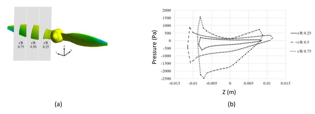
Surface pressure plot: (a) position of airfoil section, (b) pressure plot at ZX plane.
Conclusions
In this work, KG-surrogate-assisted MHOs were successfully applied for UAV propeller optimization. The design problem was defined to maximize the propeller efficiency subject to the ratio of thrust to torque at a rotating speed of 6,500 rpm. The twist angles and the ratio of blade thickness to chord length on the twenty airfoil sections of a propeller were considered as the design parameters. CFD was used to analyze the aerodynamics of the propeller, while the KG model was applied for objective and constraint function approximation. An OLHS technique was used for design of experiment to generate a set of sampling points for constructing the KG model. Several MHOs were applied while their performances were investigated. The results demonstrated that KG-DE is the most efficient method for solving propeller optimization problems. The optimal design presented a propeller efficiency that increased by about 0.6% compared with the maximum result of the best sampling point.
In future work, improving the surrogate-assisted MHO method by applying an infill sampling method and/or using hybrid surrogate models as well as multi-fidelity modelling will be studied.
Acknowledgement
This research project is supported by Rajamangala University of Technology Isan, under contract no. ENG15/65, and the National Research Council of Thailand (NRCT), under grant no. N42A650549.
Compliance with ethics guidelines
The authors declare that they have no conflict of interest or financial conflicts to disclose.
This article does not contain any studies with human or animal subjects performed by the any of the authors.