
Introduction
The transportation sector in Indonesia, especially railroads, is starting to develop rapidly, both for mass/passenger and goods transportation. Mass transportation includes Mass Rapid Transportation (MRT) in DKI Jakarta, the Jakarta-Bandung bullet train, and Light Rail Transportation (LRT), which was built in several provincial/district capitals (Surabaya, Bandung, Tangerang, Palembang). At the moment, one of the most popular train services is the Argo Parahyangan train, which serves the Bandung-Jakarta route. The train line from Bandung to Jakarta has many bends and high elevation, especially around Purwakarta. Argo Parahyangan Train engineers are required to have qualified skills so that the train trip is not only safe and comfortable but also punctual. In this context, a locomotive simulator will be beneficial to accelerate the training for locomotive drivers.
Simulation is defined as an activity imitating the behavior of operating processes in the real world all the time (over time) by Sokolowski and Banks in [1]. To perform the simulation, a model that is implemented in a simulator needs to be built. In the context of engineering or technology, simulators are used for system performance optimization, testing, safety systems, training, education, and even for entertainment. It is described by Pugi et al. in [2] that a desired mission simulation plays an important role in the optimization of train operation especially for energy efficiency. Basically, this train simulator involves the dynamics of movement, visual appearance, and sound of the environment. The dynamics of the movement consists of longitudinal translation (for going forward and backward), the dynamics of the rotational roll movement (which
Copyright ©2024 Published by IRCS - ITB ISSN: 2337-5779
J. Eng. Technol. Sci. Vol. 56, No. 3, 2024, 425-438 DOI: 10.5614/j.eng.technol.sci.2024.56.3.10
<sup>1</sup>School of Electrical Engineering and Informatics, Institut Teknologi Bandung, Jalan Ganesa No. 10, Bandung 40132, Indonesia
<sup>2</sup>Institut Teknologi Sains Bandung, Jalan Ganesha Boulevard LOT A1 CBD Kota Deltamas Tol Jakarta-Cikampek KM 37, Cikarang Pusat, Kabupaten Bekasi, Indonesia
causes a difference in the height of the left and the right side of the train), and pitch (which causes a difference in the height of the front and the rear sides of each carriage).
Until now, several researchers have conducted studies related to train dynamics modeling. The studies include: modeling of the forces between carriages; modeling of air brakes as a braking mechanism; modeling of locomotives; study of train resistance (wheel-rail relations or rolling friction); and the design of lateral/vertical ratio calculator to predict the possibility of a train leaving the rail due to the forces on the train. These models are usually represented in a nonlinear differential equation, which is called TOES (Train Operations and Energy Simulator) modeling (see Klauser [3]). In another study, by Spiryagin et al. in [4], eight teams involving ten institutions from different countries participated in conducting comparisons focusing on modeling connections between carriages among various longitudinal train dynamics simulators in China, Australia, Russia, France, and Italy.
Meanwhile, other researchers focused on modeling and calculating approaches to various input forces (Cole et al. [5]). The equation given includes force and mass relationship, coupling force (connection), lubricated friction (part of coupling and draft gear), damping modeling/force equation for polymer type draft gear. The implications for vertical and lateral stability due to the coupling force component at the bend are also discussed in this study. Crash and impact simulation on a freight train model (locomotor, carriage and coupler models are described). In addition, this study also discusses train dynamics when starting and stopping, tippler analysis (to release the carriages), as well as coupler force as a conclusion that longitudinal dynamics has significant implications for longitudinal force, acceleration, train stability, and energy consumption.
Arsahd et al. [6] derived an optimal mathematical model for making a simulator including the equation for the connection between the carriages (coupler), which depends on the coefficient of friction, speed, angle to the vertical axis. Modeling for the forces on the given track depends on the elevation gradient and the bend. The challenge faced by this researcher is the validation and verification of the values used in the simulator due to the lack of real data.
In another study by Stoklosa and Jaskiewicz in [7], a simulation study was carried out on a large tonnage freight train with two diesel locomotives and sixty freight carriages. The coupling scheme between carriages is a parallel between spring 1 and the damper, which is then serialized with spring 2 (Automatic Coupler SA-3). The rail is winding and the rail head profile is assumed to be in a straight line and worn unilaterally for sharp turns. The simulation was carried out with the Train, Train3D, and Loco modules in the Universal Mechanism v6.0 software with non-simultaneous braking of all carriages. In the middle carriage, a surge of 500 kN was detected, and in the last carriage there was also a momentary compression force of 500 kN. Such a large force can cause the carriage to come off the rails (derailment).
Andersen et al. in [8] discussed the Train Energy and Dynamics Simulator (TEDS) simulator, which is used for risk evaluation, safety, energy consumption, train operation, trip quality, and other evaluations. Longitudinal, vertical, and lateral simulations are not included. The simulated train is a simple train with one locomotive and nine carriages. In the train dynamics model, the factors considered are weight, length, track resistance characteristics, aerodynamic resistance, coupling elements, braking characteristics, tractive effort, and dynamic braking effort for locomotives.
Kovalev et al. in [9] used a longitudinal model at the time to study the process of automatically releasing cargo carriages so that the joints between the trains do not break down quickly. The simulation object with bends and inclines is a logistics train with 238 carriages. A field experiment was carried out using four carriages from a train with 238 carriages. The results of the simulation and field experiments were compared, which showed a good agreement between the two.
Xu et al. in [10] tried to find locomotive and freight train configurations that provide the minimum coupler force and the best longitudinal dynamic performance with the spring-coupler-spring connection model. Regarding the problem of load distribution, the minimum coupler force occurs when the load on each carriage is lighter than the carriage which is right in front of it. In a train model with two locomotives and five trailers, when the first locomotive is at the head of the train, then the best position of the second locomotives is at the end of the train, in which the coupler is minimum. However, the worst performance of the train longitudinal dynamics is obtained when two locomotives are positioned in the head.
Wi et al. in [11] attempted to analyze longitudinal dynamics with a newer and more detailed model of airbrake dynamics during braking as a result of the delay coupler force. The study was conducted on a freight train with 210 carriages. Braking can be done in the simulation-run of the train. The simulation results were validated with real test data on train trips.
Van de Merwe and le Roux in [12] presented a simulation model of a locomotive, which includes the longitudinal, vertical, pitch, and wheelset rotational dynamics, which are the most important aspects for wheel slip control. The researchers then developed an estimation model based on this simulation model. The results showed that accurate and fast estimation of the adhesion force of the individual wheelsets could be achieved.
Researchers in [13] proposed three prediction models for locomotive traction energy consumption. The models are constructed based on a large number of measured operation data of the HXD1 locomotive, in order to accurately measure and predict the energy consumption of locomotive traction. In this paper, the three models are compared, and it is proven that the Support Vector Machine (SVM) algorithm achieves better prediction accuracy and overall performance than the Radial Base Function (RBF) and the Backpropagation algorithm.
Bosso, Magelli and Zampieri in [14] proposed the simulation of the longitudinal train dynamics using the multibody software Simpack, with the additional dedicated in-house code developed in MATLAB. The authors used the longitudinal model by adding extra resistant forces to represent the track curvature and gradients. to model coupling elements, look-up tables of the data from experimental tests were used. The model was then validated according to the benchmark inputs and compared with the outputs from other researchers.
The main contribution of the present paper is a longitudinal dynamics model that was specifically developed for the CC203 or CC204 locomotive. This is a type of locomotive that is used for the Argo Parahyangan regular train from Bandung to Jakarta and vice versa in Indonesia. The CC204 locomotive has essentially the same traction force characteristics as CC203. The difference is merely in the driver cabin, where CC204 has two driver cabins so that there is no need to commutate the locomotive for each return trip. The parameters of the model were taken from the locomotive and train physical characteristics and from the literature. Due to the absence of traction force measurement, the traction characteristic of the CC203 locomotive was used to calculate the locomotive traction force based on the train's measured speed time history during one trip. The model was then validated by running one trip simulation and the simulation's result was compared to data of a real train trip.
Simulation Architecture
We designed the simulator with the following specifications:
- 1. Train vehicle model
- a. Traction: single locomotive
- b. Wagon: multiple wagon (passenger or freight)
- 2. Motion platform simulator: 4 degrees-of-freedom (DoF)
- a. Lateral: maximum displacement: ±100 mm, maximum velocity: 200 mm/s
- b. Longitudinal: maximum displacement: ±100 mm, maximum velocity: 300 mm/s
- c. Roll: maximum displacement: ±20°, maximum velocity: 20°/s
- d. Pitch: maximum displacement: ±20°, maximum velocity: 20°/s
- 3. Driver interface
- a. Virtual view: front, rear, and side scene
- b. Train trip: Jakarta Bandung (round trip)
- c. Physical instrument: hand pedal levers (throttle, dynamic brake, service brake)
- d. Virtual instrument: input buttons, output indicator, programmable metering
The architecture of the Loco Pilot Simulator is as depicted in Figure 1, consisting of a physical interface (throttle and brake levers), which connects the simulator with the driver in-training (driver action) in the cabin of the 3/4 axis mechanical platform. The simulator was designed to maximize the real experience and hence it is also equipped with visual environment and sounds effects. The mechanical platform is driven by motion controller through actuators, gearbox, and mechanical transmission. The I/O monitoring, Dynamic Train Generator, Visual Database computers, and motion control computers exchange data accordingly through a data network. Meters and indicators in the locomotive were also installed in the driver's cabin as in the real locomotive cabin.
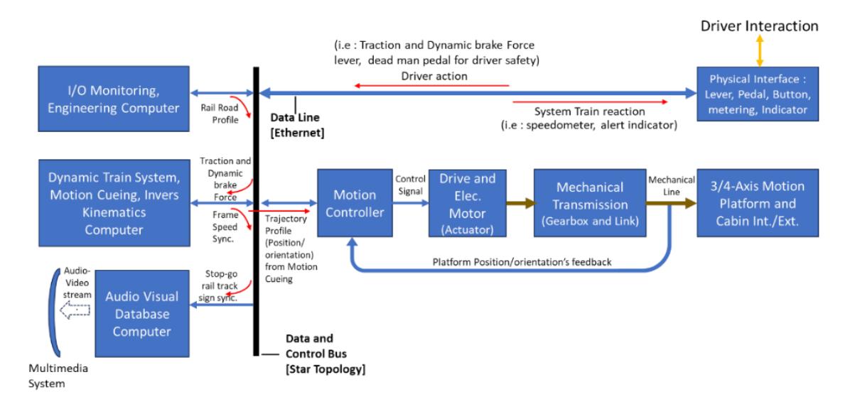
Loco pilot simulator architecture.
The driver action, through throttle and brake levers, acts as an input of the Dynamic Train System Generator to generate position and velocity data of the locomotive (Figure 2). In the system generator, all drag forces, i.e., brake resistance (Fb), curving resistance (Fcr), propulsion (roll and air) resistance (Fpr), and grade resistance (Fg) forces, are mathematically modeled using suitable parameters (such as railway friction coefficient μ) and computed. Curve and grade (slope) profiles may also be computed based on train's current position, which provides range, radius, and inclination (o /oo) data. The position s(t) and velocity v(t) of the locomotive were derived from the mathematical model of the longitudinal locomotive dynamics, which will be described in the following section.
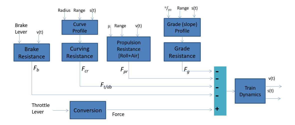
Dynamic train system generator.
Longitudinal Locomotive Dynamics Model
Model Formulation
A train may be modeled as a simple mechanical model consisting of several masses, springs, and dampers (Davydov and Keyno in [15] and Zhou et al. in [16]). In this case, a locomotive and two railroad carriages (or wagons) are assumed to be lumped masses, while the connections between carriages are modeled by a parallel spring-damper system, as depicted in Figure 3 with variables and parameters as defined in Table 1.
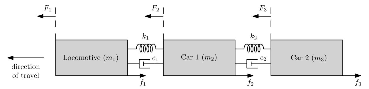
Simplified mechanical model of a locomotive and two carriages.
| Variable | Definition | Unit |
|---|---|---|
| 𝑚1, 𝑚2, 𝑚3 | Mass of locomotive, carriage 1, and carriage 2 | kg |
| 𝑣1, 𝑣2, 𝑣3 | Velocity of locomotive, carriage 1, and carriage 2 | m/s |
| 𝑥1, 𝑥2, 𝑥3 | Longitudinal position of locomotive, carriage 1, and carriage 2 | m |
| 𝐹1, 𝐹2, 𝐹3 | Force acts on locomotive, carriage 1, and carriage 2 | N |
| 𝑓1, 𝑓2, 𝑓3 | Friction force acts on locomotive, carriage 1, and carriage 2 | N |
| 𝑐1 | Damping coefficient between locomotive and carriage 1 | Ns/m |
| 𝑐2 | Damping coefficient between carriage 1 and carriage 2 | Ns/m |
| 𝑘1 | Spring constant between locomotive and carriage 1 | N/m |
| 𝑘2 | Spring constant between carriage 1 and carriage 2 | N/m |
| 𝑔 | Gravitational acceleration | m/s2 |
Table 1 List of variables and parameters.
Equation of Motion
Applying the second Newton's law on Figure 4 (a), the differential equation of motion (EoM) on mass 1 can be derived as in Eq. (1).
\[F_1 - f_1 - k_1(x_1 - x_2) - c_1(\dot{x}_1 - \dot{x}_2) = m_1 \ddot{x}_1\] \[m_1 \ddot{x}_1 + c_1 \dot{x}_1 + k_1 x_1 - c_1 \dot{x}_2 - k_1 x_2 = F_1 - f_1\] (1)
From Figure 4 (b), the EoM on mass 2 can be derived as in Eq. (2).
\[F_2 - f_2 - k_1(x_2 - x_1) - c_1(\dot{x}_2 - \dot{x}_1) - k_2(x_2 - x_3) - c_2(\dot{x}_2 - \dot{x}_3) = m_2 \ddot{x}_2\] \[m_2 \ddot{x}_2 + c_1(\dot{x}_2 - \dot{x}_1) + c_2(\dot{x}_2 - \dot{x}_3) + k_1(x_2 - x_1) + k_2(x_2 - x_3) = F_2 - f_2\] (2)
Lastly, the EoM on mass 3 is obtained from Figure 4 (c) as in Eq. (3).
\[F_3 - f_3 - k_2(x_3 - x_2) - c_2(\dot{x}_3 - \dot{x}_2) = m_3 \ddot{x}_3\] \[m_3 \ddot{x}_3 + c_2(\dot{x}_3 - \dot{x}_2) + k_2(x_3 - x_2) = F_3 - f_3\] (3)
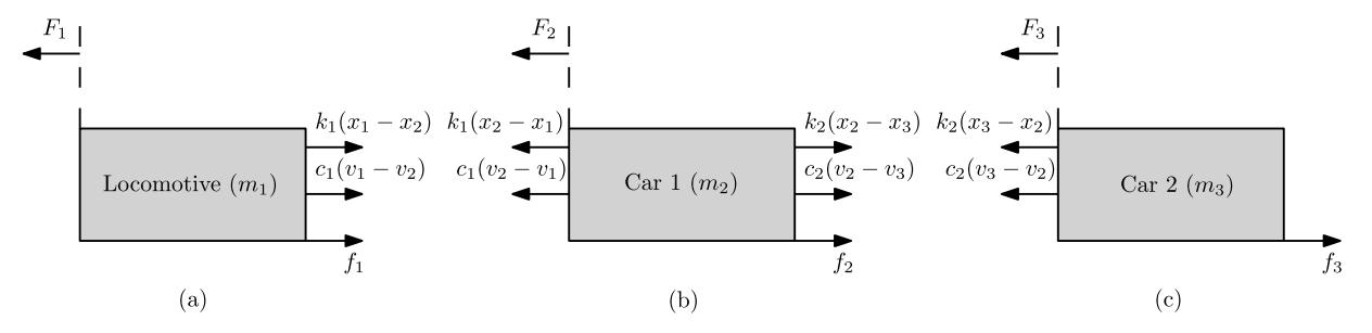
The free body diagram on (a) mass 1; (b) mass 2; and (c) mass 3.
The friction forces that acts on the masses, , with = 1, 2, 3, consist of several friction forces, defined as in Eq. (4).
\[f_i = f_{s,i} + f_{a,i} + f_{b,i} + f_{c,i} + f_{d,i}\] (4)
where , is the friction force between the locomotive/carriage and the railroad, , is the aerodynamic drag force, , is the gradient resistance, , is the curve resistance, and , is the acceleration resistance.
Acting Forces
The friction force between the locomotive/carriage and the railroad is defined as in Eq. (5).
\[f_{s,i} = \mu_i m_i g \tag{5}\] where is the friction coefficient, is the respective mass, and is the gravitational acceleration.
The aerodynamic drag force for the locomotive, , , and carriages, , , = 2, 3, are defined as in Eq. (6a) and (6b).
\[f_{a,1} = \left\{ 2.86 + 0.55 \frac{F_1}{m_1} \left( \frac{v_1 + v_{a,1}}{10} \right)^2 \right\} m_1 \times 10^{-3}\] (6a)
\[f_{a,2} = \left\{ 2.5 + \left( \frac{v_i + v_{a,i}}{K_i} \right)^2 \right\} m_i \times 10^{-3}\] (6b)
where 1 is the cross-sectional area of the locomotive (m2), , is the wind speed (km/h), and is the carriage constant.
Using the model in Figure 5 and by assuming that the gradient angle is small, i.e., sin ≈ tan ≈ , the gradient resistance , is defined as in Eq. (7).
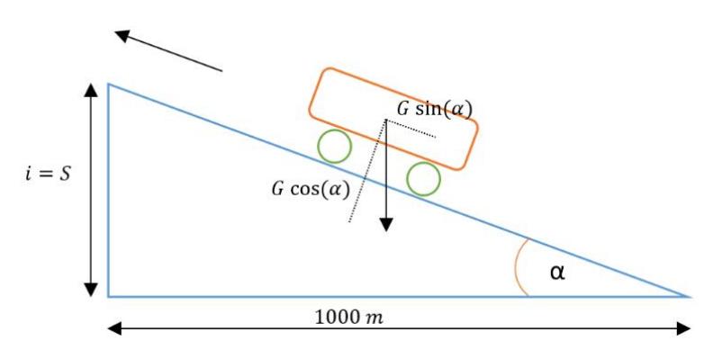
The gradient resistance model.
\[f_{b,i} = s_i m_i \tag{7}\] where is the height of the gradient.
The curve resistance , is defined as in Eq. (8).
\[f_{c,i} = \left(\frac{400}{R_i - 20}\right) m_i \times 10^{-3} \tag{8}\] where is the corner radius (m).
The acceleration resistance , is defined as in Eq. (9).
\[f_{d,i} = \left\{ \frac{1000}{9.81} \ddot{x}_i (1 + c_i) \right\} m_i \times 10^{-3}\] (9)
where is the additional inertial factor during rotation.
Data, Model Identification, and Simulation Results
Data
Modeling was carried out based on using real data from the Jakarta-Bandung track (Figure 6) that was collected using a handheld GPS, consisting of altitude and longitude of the train at each measurement time of one second. The real data was then processed to derive required specific data for system modeling. Raw data of distance change at each time is plotted in Figure 7 (a), which was filtered using a low-pass filter to produce smoother data (Figure 7 (b)). The distance (relative to the departing station) data was then obtained as shown in Figure 8. Figure 9 (a) and 9 (b) show raw data and filtered data of speed as a function of time, respectively. The altitude as a function of time is also depicted in Figure 10. Meanwhile, due to the unavailability of a traction force sensor, the traction force of the locomotive was back-calculated from the speed using the torque-speed characteristic of the CC203/CC206 locomotive. Figures 11 (a) and (b) present traction force as a function of time, and traction force as a function of speed (reproduced force-speed characteristic of the locomotive), respectively.
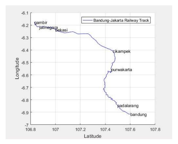
Jakarta-Bandung track.
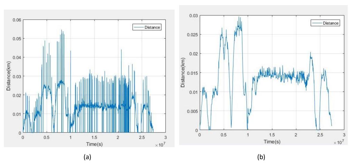
Distance vs time: (a) unfiltered; (b) filtered.
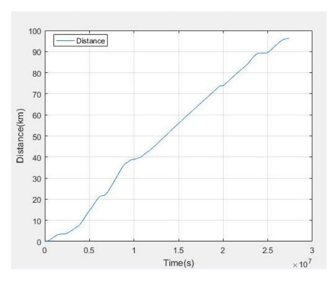
Distance vs time.
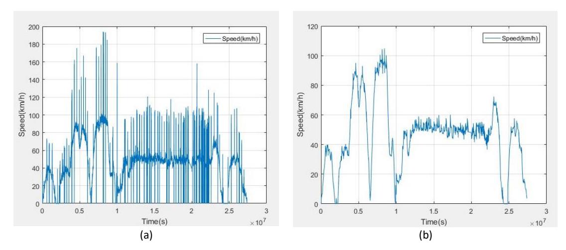
Speed vs time: (a) unfiltered; (b) filtered.
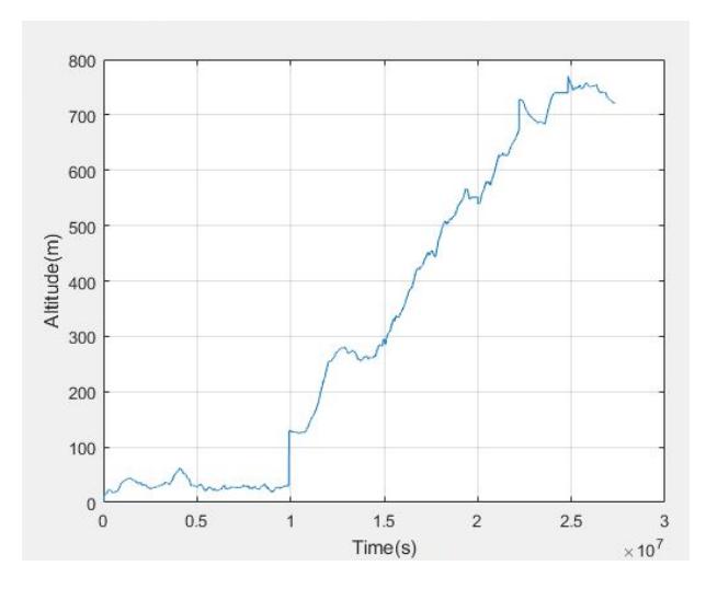
Altitude vs time.
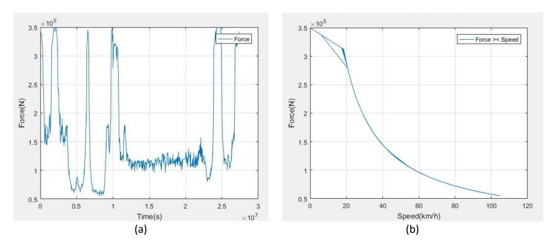
Traction force as a function of: (a) time; (b) speed.
Model Identification
From the data collection process for the Jakarta-Bandung train journey, a series consisting of distance change data for each time sampling, instantaneous altitude, and instantaneous speed were obtained. The data was obtained for 7,416 seconds with a sampling time of 1 second. These three types of data were filtered and processed so that they became input and output quantities for system identification. From the processing of the distance change data, the following mileage profile was obtained (see Figure 12). In 7,415 seconds, a distance of 9.7494 × 10⁴ m, approximately 97.5 km, was covered. Meanwhile, the drag force plot due to the difference in height (incline) was obtained from processing the instantaneous altitude data, as depicted in Figure 13.
Using the information of the friction coefficient of a stainless-steel wheel against a stainless-steel rail, the sum of all friction forces was calculated as depicted in Figure 14. On the other hand, the amount of force that must be generated by the locomotive to move was computed based on the instantaneous speed data and the torquespeed characteristic of the CC203/C206 locomotive. The estimated position of lever/notch was then obtained as depicted in Figure 15.
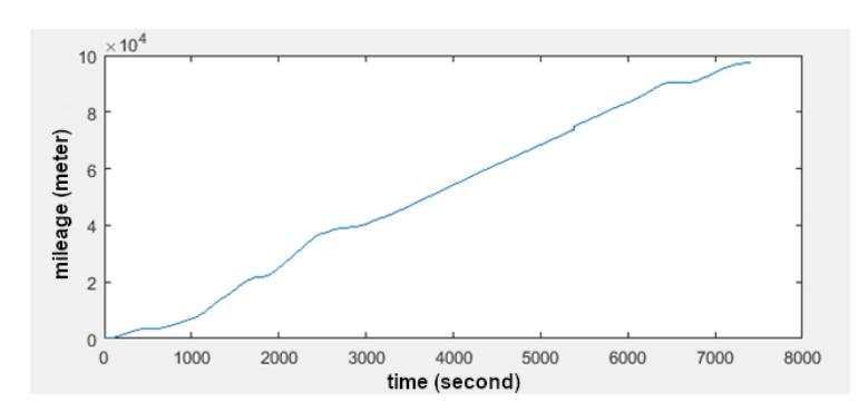
Mileage profile.
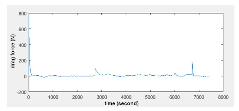
The drag force due to the difference in height (incline).
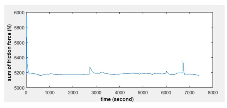
Sum of friction forces.
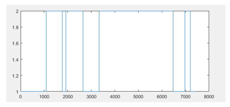
Estimated position of lever/notch.
Due to unknown railroad carriage parameters of the simple mechanical model, we took a black box approach for system identification for the model dynamics (see Eqs. (1), (2), and (3)), where F1 is the locomotive traction force, F2 = F3 = 0, f1 = fi (Eq.(4)) and f2 = f3 = 0. Instead of a first order model as reported by Syahira et al. in [17], the identification of the system was carried out based on a second-order model. In this case, two railroad carriages in the mechanical model were assumed to be one lumped mass. For this identification process, 70% of the measured data were used. In the model, the traction force that needs to be generated by the locomotive is taken as the second input (F1), the total force (fi of Eq. (4)) of the incline's drag force Eq. (5) and the friction force Eq. (7) was taken as the first input. In train operation, information on position and time are of importance since they determine operation cost, safety, and punctuality. The position or mileage of the train from the departing station was therefore chosen as the output of the model. Note that other opposing forces in Eqs. (6), (8), and (9) were assumed small and then neglected. The linear and continuous-time state space model was obtained using MATLAB with the following system matrices:
\[A = \begin{bmatrix} 0 & 1 \\ -5.6 \times 10^{-7} & -2.3 \times 10^{-3} \end{bmatrix}, B = \begin{bmatrix} 4.8 \times 10^{-6} & -1.18 \\ 10^{-5} & -0.22 \end{bmatrix}, C = \begin{bmatrix} 1 & 0 \end{bmatrix}, D = \begin{bmatrix} 0 & 0 \end{bmatrix}\] (10)
The model was then validated with the remaining 30% data in terms of the position of the train; the mileage result is depicted in Figure 16. The figure shows a Root Mean Square Error (RMSE) of 812.0152 m with a mean equal to 86182 m, i.e., a model error of 0.94%. In addition, a further model validation was performed by running a simulation along the route for 7,415 s, where resultant force data acting on the train was fed to the model. The mileage result from the simulation is shown in Figure 17. With respect to 70% of the data, the RMSE of the simulation was 693.1709 m with a mean equal to 49753 m, i.e., a model error of 1.39%. Another model validation by simulation run was undertaken but now using slope profile data (from real instantaneous elevation data) as input for incline drag, frictional information, and predicted lever position. The mileage result was obtained as shown in Figure 18. The RMSE was obtained as 2940.7 m with a mean equal to 49753 m, i.e., a model error of 5.91% (model fitness level = 94.09%).
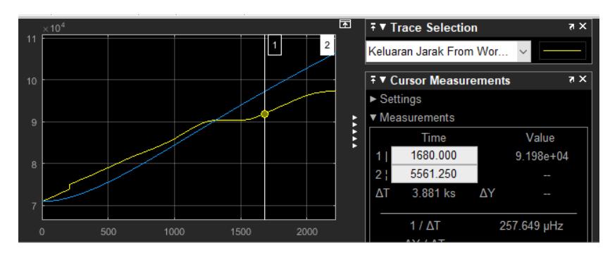
Mileage validation using 30% data.
Mileage validation using 70% data.
Mileage validation using 70% data, incline profile, friction forces, and lever position.
Simulation Results
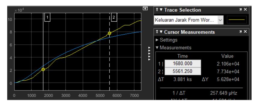
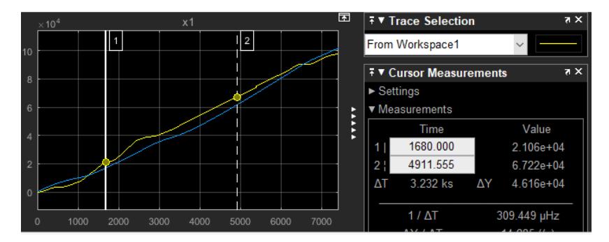
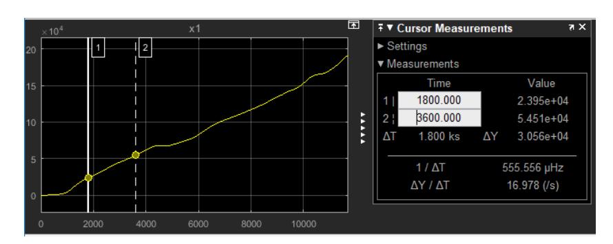
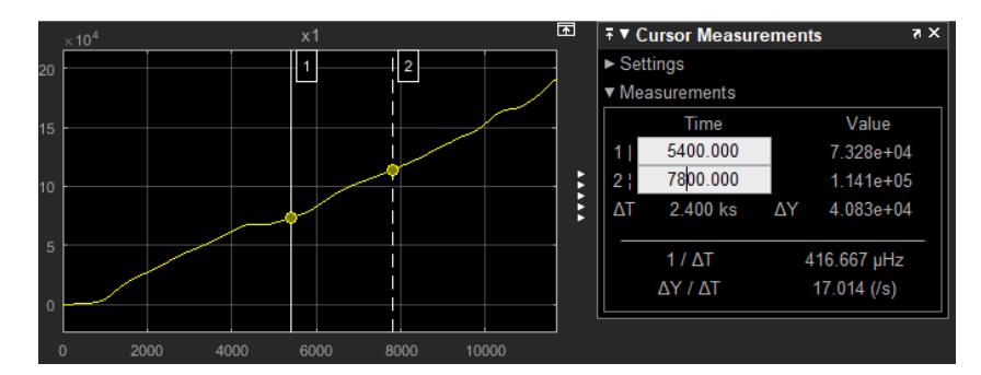
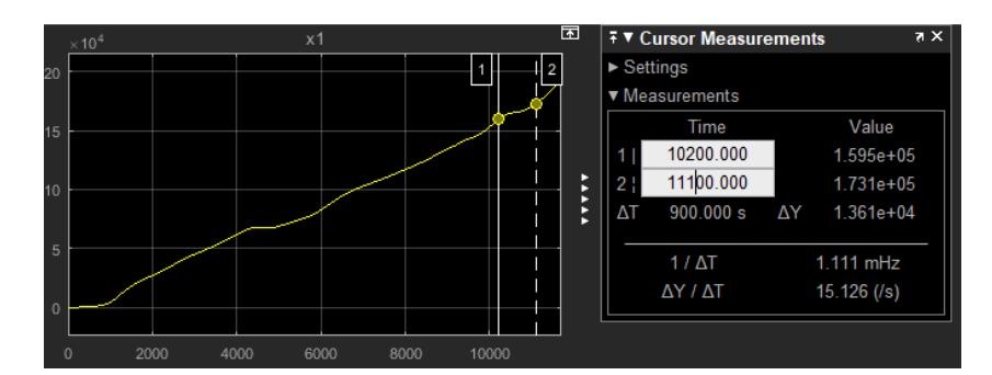
Having validated the model, it was used in the simulation in MATLAB with a simulation time of 195 mins (= 11,700 s). The simulation results were compared with the real collected data, where a resampling was performed from the 7,416 available data points to produce 11,700 data points, with a time sampling of 1 s. Assuming a trip from Gambir station (Jakarta) to Bandung, the comparison between actual trip scenarios and simulation results for seven different observation-times is presented in Table 2 and the mileage simulation results are shown in Figure 19 to Figure 22. Table 2 shows that the simulation of a complete trip from Gambir Station (Jakarta) to Bandung resulted in a mileage difference of 11.1 km from the real distance of 203 km, a difference of 5.47%.
| Travel Time | Actual Data | Simulation Result | Difference |
|---|---|---|---|
| 30 mins (Gambir-Bekasi) | 19.00 km | 23.95 km | +4.95 km |
| 60 mins (Bekasi-Purwakarta part 1) | 38.00 km | 54.51 km | +16.51 km |
| 90 mins (Bekasi-Purwakarta part 2) | 80.50 km | 73.28 km | -7.22 km |
| 130 mins (Purwakarta-Cimahi part 1) | 143.83 km | 114.1 km | -29.73 km |
| 170 mins (Purwakarta-Cimahi part 2) | 177.16 km | 159.5 km | -17.66 km |
| 185 mins (Purwakarta-Cimahi part 3) | 194.66 km | 173.1 km | -21.56 km |
| 195 mins (Cimahi-Bandung) | 203 km | 191.9 km | -11.1 km |
Table 2 Comparison between actual data and simulation results.
Mileage simulation from 30 to 60 minutes of travel time.
Mileage simulation from 90 to 130 minutes of travel time.
Mileage simulation from 170 to 185 minutes of travel time.
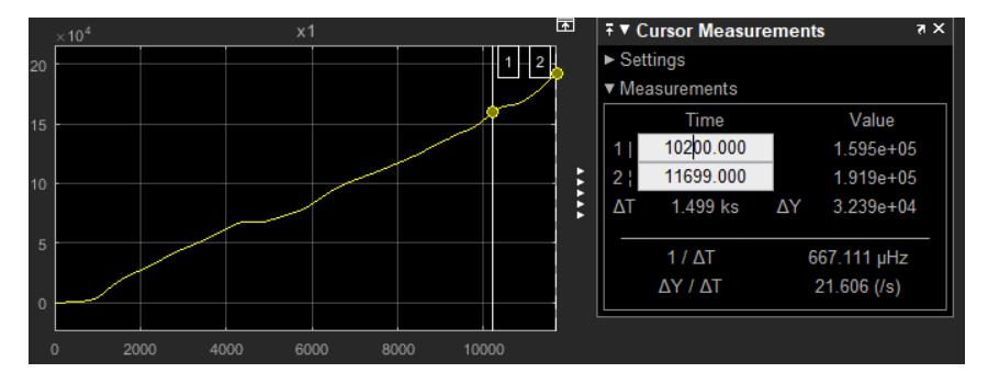
Mileage simulation from 170 to 195 minutes of travel time.
Concluding Remarks
This paper presented the development of longitudinal train dynamics model that may be used in Loco Pilot Simulator for driver training. Specifically, the model was developed for the Argo Parahyangan train that travels from Jakarta to Bandung in Indonesia. As an initiative effort of train modeling in Indonesia, based on a derived physical model of a two-wagon train, a second-order linear time invariant model was therefore considered
sufficient and obtained based on real measurement data from of the train trip with a CC203/C204 locomotive. After model validation using 30% and 70% of the real data, a simulation was run by using slope profile data (from the real instantaneous elevation data) as input for incline drag, frictional information, and predicted lever position. In this case, a model fitness level of 94.09% was obtained. To further validate those results, we performed a simulation using the model with a simulation time of 195 minutes. The simulation of a complete trip from Gambir Station (Jakarta) to Bandung resulted in a mileage difference of 11 km from the real distance of 203 km. Some assumptions were made in this study; future work will be focused on the improvement of the model by considering the control actions performed by the train driver to obtain a more accurate model.
Compliance with ethics guidelines
The authors declare that they have no conflict of interest or financial conflicts to disclose.
This article does not contain any studies with human or animal subjects performed by any of the authors.