
Introduction
Data acquisition (DAQ) is an indispensable feature for applications, especially Internet of Things (IoT) applications where data (i.e., signals from sensors) are acquired simultaneously. Different data types of interest can be collected by a great number of data acquisition systems. Rosiek et al. [1] built a meteorological data collection system using an ATMEGA16 microcontroller unit (MCU) to get data from sensors and send it back to users via the internet. Boquete et al. [2] proposed a driving data logging model to collect the location, speed, driving behavior, and number of passengers and send it to the control center through the internet. DAQ systems for solar-powered devices using MCUs linked with various sensors have also been developed [3, 4]. The building temperature acquisition system proposed in [5], which uses various low-cost temperature sensors controlled by a low-cost Arduino kit, demonstrates the effectiveness of MCU-based DAQ systems. In 2019, Babiuch et al. [6] developed a data logging and processing system based on the ESP32 MCU, where the collected data is displayed on an on-board display. MCU-based DAQ systems are typical, but there is a lack of research concentrated on evaluating the ability of the MCU to acquire data and access recorded data.
The combined infrastructure between artificial intelligence (AI) and IoT is named Artificial Intelligence of Things (AIoT), in which the AI model intends to be standalone executed on edge devices. AIoT is gaining popularity due to the advent of tiny machine learning (tinyML) architectures that aim to run machine learning (ML) models on resource-limited MCUs. TinyML models are applied to integrate classification applications directly on edge devices. The designing and training of these tinyML models entail collecting and processing data from different types of sensors, such as rotation angles [7-9], sounds from analog or digital micro [9-13], and ultrasonic waves,
Copyright ©2024 Published by IRCS - ITB J. Eng. Technol. Sci. Vol. 56, No. 4, 2024, 474-488 ISSN: 2337-5779 DOI: 10.5614/j.eng.technol.sci.2024.56.4.4
Faculty of Automation Technology, College of Engineering, Can Tho University, 3/2 street, Can Tho city 94100, Vietnam
2Aerospace Engineering and Aviation Discipline, School of Engineering, RMIT University, La Trobe street, Melbourne, VIC 3000, Australia
3Deparment of Electrical Engineering and Energy, College of Electrical Engineering - Electronic - Telecommunications, Can Tho University of Technology, Nguyen Van Cu street, Can Tho city 94100, Vietnam
vibration [9], etc. Accurate gathering of these sources is critical to providing a reliable source of data for the design process, operation, and lifting of the ML models for edge devices.
In addition, the implementation of pre-processing procedures such as fast Fourier transform (FFT) analysis, digital filtering, wavelet filtering, and image processing directly on the MCUs is crucial to serving embedded applications in general and IoT/AIoT in particular. Typically, in 2011, Rein and Reisslein [14] proposed a technique to compress images from image sensors using low-memory wavelet transform techniques on 16-bit MCUs with limited random-access memory (RAM). In 2016, Mirghani [15] implemented a finite impulse response (FIR) digital filter on an Intel 8051 chip that filters radar signals. Similarly, in 2022, Tey and colleagues applied a digital filter to pre-process audio signals before converting them to spectrogram images and utilizing them to train deep learning networks [16]. Next, in 2019, Warden and colleagues applied an algorithm to convert audio data to spectrogram images using the FFT and Mel-frequency cepstral coefficient (MFCC) functions provided by the TensorFlow Lite library to implement speech recognition applications on Arduino boards and some other microcontrollers [17, 18]. These studies imply that a time-frequency domain image conversion algorithm is necessary but there is no general algorithm available to readily apply it to other applications.
Cost is a top criterion for IoT/AIoT systems where numerous edge devices are deployed, so directly applying a built-in analogue to digital converter (ADC) on low-cost MCUs to sampling data is a practical solution. Directly utilizing the built-in ADC module could reduce the number of additional circuits, thereby making the system lean, reducing energy consumption, and optimizing the cost. However, the ADC module still has some limitations in acquiring data, such as a low sampling rate and requiring better central processing unit (CPU) performance. The built-in I2S module of the ESP32 MCU provides the feature of automatically streaming data from the ADC module to the memory at a specific sampling rate. The feature could relieve the CPU's performance and easily scale up the sampling rate. However, not enough studies have concentrated on evaluating this solution.
This study proposes a solution to overcome the limitation of the data acquisition speed of the ADC module, which depends on the processing ability of the CPU, by combining the I2S and ADC modules of an ESP32- WROOM-32 MCU. The I2S module has high-speed data acquisition capabilities that can automatically collect the converted samples from the ADC module into DMA's buffer without requiring CPU performance. Sine waves generated at different frequencies and white noise are sampled by the proposed feature and stored on a personal computer (PC) for analysis. The frequency domain of these data is obtained by applying the FFT to assess the accuracy of the data and generated noise. Digital filtering algorithms (i.e., low-pass filter, high-pass filter, and band-pass filter) are proposed to remove the noise generated in the collected data. The low-pass filter is used to remove high-frequency noise, while the high-pass filter removes low-frequency noise. The band-pass filter simultaneously removes the frequency noise around the original frequency of the signal. Furthermore, a time-frequency domain imaging algorithm is proposed as a solution for directly pre-processing data on the MCU, which can be applied to the TinyML network on embedded devices. These algorithms are an important prerequisite for future studies, especially applications of deploying tinyML models on resource-constrained MCUs.
The main contributions of this study are:
- 1. Proposing a data acquisition solution based on the combination of ADC and I2S modules integrated on the ESP32-WROOM-32 MCU.
- 2. Providing digital filtering algorithms, i.e., low-pass filter, high-pass filter, and band-pass filter, that are suitable for deployment on embedded systems because of their fast and good response.
- 3. Modifying and implementing a spectrum image generation algorithm for converting the acquired data into images directly in the embedded systems.
The remainder of the paper is organized as follows: the sections on data collection and methodology provide a description of the system and methods used in the study, including digital filtering algorithms and spectrum image generation algorithms. The results and discussion section presents the experimental results and their discussion. Finally, the conclusion section concludes the article with a summary of the findings and future research directions.
Data Collection and Methods
Experimental Configuration
The sine waves used in the experiment was generated by the NI VirtualBench All-In-One instrument and the white noise signal was created by the Soundcard Scope software. The sine waves were generated at a number of different frequencies, including 0.1 kHz, 1 kHz, 4 kHz, 8 kHz, 16 kHz, and 20 kHz. The white noise was transmitted at a frequency of 20 kHz. These signals were sampled by the ESP32 and stored on a PC at sampling frequencies of 16 kHz, 44.1 kHz, and 96 kHz.
When converted to the frequency domain, a single sine wave has only one single frequency value. Therefore, the generated noise during data acquisition by the proposed feature can be easily detected using FFT analysis. The FFT converts recorded data into the frequency domain. The accuracy of the received signal was evaluated by determining the number and amplitude of frequencies that differed from the frequency of the original signal. White noise contains all the frequencies when converted to the frequency domain. Thus, it was used to evaluate the ability of the proposed feature to collect complex signals.
ADC Module and I2S Module on ESP32
An analog-to-digital converter (ADC) is used to convert an analog signal to digital format for embedded systems. The ADC is a useful tool that helps embedded systems collect information about the external world. The input signal is typically an analog voltage from the sensors. In ESP32, the ADC conversion results provided by the ADC driver APIs are raw data. The resolution of the ESP32 ADC raw results under single-read mode is 12-bit, with the digital output result standing for the voltage. However, because the ADC-RTC mode commonly used in the ESP32 has a low sampling rate, it is unsuitable for high-frequency sampling operations. Therefore, the ADC module needs to be combined with the I2S module, which has a dedicated DMA controller that allows for streaming sample data without requiring the CPU to copy each data sample.
Two digital audio devices can stream audio data via a synchronous serial communication protocol called I2S (Inter-IC Sound) [19]. The data flow on this bus must be high-speed and continuous so as not to affect the audio quality. The I2S bus has a reliable speed controlled by DMA peripherals, which does not require too much MCU time. The ESP32 consists of two I2S peripherals that can be set up for importing and exporting data sets by I2S drivers. The interface pins corresponding to I2S's communication modes are detailed in Table 1.
| Communication mode | Data pin | Function | ||
|---|---|---|---|---|
| Standard mode or TDM | MCLK | Master clock line. This is an optional signal | ||
| that depends on the slave side and is mainly | ||||
| used for offering a reference clock to the | ||||
| I2S slave device. | ||||
| BCLK | Bit clock line. The bit clock for the data line. | |||
| WS | Word (slot) select line It is usually used to | |||
| identify the vocal tract, except in PDM | ||||
| mode. | ||||
| DIN/DOUT | Serial data input/output line. (Data will loop | |||
| back internally if din and dout are set to the | ||||
| same GPIO). | ||||
| CLK | PDM clock line. | |||
| PDM | DIN/DOUT | Serial data input/output line. | ||
Table 1 Communication modes of I2S protocol and data pins [19].
The I2S driver can configure each I2S controller, which has three characteristics, i.e., master system operator, transmitter acting, and streaming data sets via the DMA controller without copying each data set. A simplex communication mode can be used by each controller. Hence, full-duplex communication is formed by merging the two controllers.
In addition, LCD mode is supported by I2S peripherals to transfer data via a parallel port using several camera modules and LCD monitors. The operating modes of LCD mode contain ADC/DAC, slave receiving camera, and primary transmitted LCD. The ADC/DAC mode is supported by the I2S0 module, which is connected to the integrated ADC/DAC module on the chip as depicted in Figure 1.
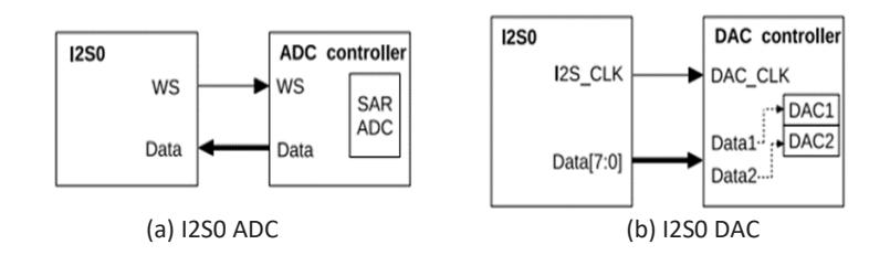
I2S0 ADC/DAC connection interface [19].
Experimental Layout
The experimental layout consisted of an ESP32 board that was connected to the signal sources via a GPIO32 and to a laptop using a USB cable, as shown in Figure 2. Each type of signal was collected every one second on the microcontroller and then sent to the laptop for storage. Five-second data samples of each data type were stored in separate files for later processing.
Experimental layout.
Implementation of Signal Processing Algorithms on Microcontroller
Fast Fourier Transform
A prominent digital signal and image processing tool is the discrete Fourier transform (DFT), but it is hardly being used due to its complicated calculation [20]. In 1965, a fast algorithm to compute DFT that significantly minimized the amount of numerical performance was proposed by Cooley and Tukey [21]. Their proposal added momentum to improving high-speed data processing algorithms according to the fast Fourier transform (FFT). DFT is represented in Eq. (1):
\[X_k = \sum_{k=0}^{N-1} A(k) W^{jk}\], j = 0, 1, ..., N-1 (1)
where A(k) are complex numbers and W is the principal N-th root of unity, which is expressed as:
\[W = e^{2\pi i/N} \tag{2}\]
The Fourier transform according to the above formula requires O(N2 ) calculations (a complex multiplication followed by a complex addition). O(N2 ) means that the time complexity of the algorithm increases linearly and exponentially with input (N). However, the FFT algorithm only takes O(N log N) calculations to produce the same result [21], leading to MCU applications. This means that the algorithm's running time increases not only linearly with input size (N) but also logarithmically. Thus, the time complexity of the algorithm is significantly improved. In this study, a fixed-point FFT is used and calculated by the KISS FFT algorithm [22], based on a C-language opensource library. This library has been integrated into the TensorFlow Lite library.
Implementation of Digital Filters
The received signal is filtered by digital filters (i.e., low-pass, high-pass, and band-pass filters) to remove unwanted noise. The low-pass filter is used to remove high-frequency noise. In contrast, the high-pass filter removes low-frequency noise. The band-pass filter simultaneously removes frequency noise around the original frequency of the signal. The transfer function (TF) of the digital filter is designed according to the infinite impulse response (IIR) technique with an order of n as follows [23]:
\[H(z) = \frac{B_{(z)}}{A_{(z)}} = \frac{b_0 + b_1 Z^{-1} + \dots + b_N Z^{-n}}{1 + a_1 Z^{-1} + \dots + a_N Z^{-n}}\] (3)
A different version of Eq. (3) can be calculated as:
\[Y_k = \sum_{n=0}^{L} b_n \, x_{k-n} - \sum_{n=0}^{L} a_n \, y_{k-n} \tag{4}\] where \(a_n\) and \(b_n\) are the coefficients of the filter, and \(x_{k-n}\) and \(y_{k-n}\) represent the values of input and output at time k-n. The correlation of the input and output of the IIR filter is shown in the following formula:
\[y[n] = b_0 x[n] + b_1 x[n-1] + \dots - a_1 y[n-1] - a_2 y[n-2] - \dots\] (5)
where y(n) is the output, x(n) is the input, and b(n) and a(n) are the coefficients of the filter. In this study, the low-pass and high-pass filters had an order of 4 and the band-pass filter had an order of 2. The n<sup>th</sup>-order Butterworth polynomial can be written as [26]:
\[B_n(s) = \sum_{k=0}^n \alpha_k \, s^k \tag{6}\] with its coefficient \(a_k\) is given by the following recursion formula [25,26]:
\[\alpha_{k+1} = \frac{\cos(k\gamma)}{\sin((k+1)\gamma)} \alpha_k \tag{7}\] where \(\alpha_0 = 1\), \(\gamma = \frac{\pi}{2n}\), and k = 0, 1, ..., n - 1. The coefficients of the 4<sup>th</sup>-order Butterworth polynomial with n = 4 are \(\alpha_0 = 1\), \(\alpha_1 = 2.6231\), \(\alpha_2 = 3.4142\), \(\alpha_3 = 2.6231\), and \(\alpha_4 = 1\). The n<sup>th</sup>-order Butterworth low-pass filter TF with \(\omega_c = 1\) can be expressed in Eq. (8) as follows:
\[(s) = \frac{1}{B_n(s)} = \frac{1}{\sum_{n=0}^{\infty} \alpha_k \cdot s_k}\] (8)
The n<sup>th</sup>-order Butterworth polynomial with a cut-off frequency \(\omega_c\) can be written as in Eq. (9):
\[B_n(s) = \sum_{k=0}^n \alpha_k \left(\frac{s}{\omega_c}\right)^k = \sum_{k=0}^n c_k s^k\] (9)
with \(c_k=\frac{a_k}{\omega_c^k}\). This implies that a 4<sup>th</sup>-order filter continuous TF as in Eq. (10) is needed:
\[H(s) = \frac{1}{c_0 + c_1 s + c_2 s^2 + c_3 s^3 + c_4 s^4} \tag{10}\]
Utilizing Tustin's method (i.e., bilinear transform) [24], set \(s = \frac{2}{\Delta t} (\frac{1-z^{-1}}{1+z^{-1}})\), then substitution of \(c_k = \frac{a_k}{\omega_c k}\) and \(\beta = \omega_c \Delta t\), the discrete TF of the 4<sup>th</sup>-order Butterworth low-pass filter H(z) with cut-off frequency \(\omega_c\) is derived from Eq. (11).
\[H(z) = \frac{b_0 + b_1 z^{-1} + b_2 z^{-2} + b_3 z^{-3} + b_4 z^{-4}}{1 + a_1 z^{-1} + a_2 z^{-2} + a_3 z^{-3} + a_4 z^{-4}}\](11)
Its coefficients are shown below
\[a_{1} = (4\alpha_{0}\beta^{4} + 4\alpha_{1}\beta^{3} - 16\alpha_{3}\beta - 64\alpha_{4})/D\] \[a_{2} = (6\alpha_{0}\beta^{4} - 8\alpha_{2}\beta^{2} + 96\alpha_{4})/D\] \[a_{3} = (4\alpha_{0}\beta^{4} - 4\alpha_{1}\beta^{3} + 16\alpha_{3}\beta - 64\alpha_{4})/D\] \[a_{4} = (\alpha_{0}\beta^{4} - 2\beta^{3} + 4\alpha_{2}\beta^{2} - 8\alpha_{3}\beta + 16\alpha_{4})/D\] \[b_{0} = \beta^{4}/D, b_{1} = 4\beta^{4}/D, b_{2} = 6\beta^{4}/D, b_{3} = 4\beta^{4}/D, b_{4} = \beta^{4}/D\] \[D = \alpha_{0}\beta^{4} + 2\alpha_{1}\beta^{3} + 4\alpha_{2}\beta^{2} + 8\alpha_{3}\beta + 16\alpha_{4}\] with \(\alpha_0 = 1\), \(\alpha_1 = 2.6231\), \(\alpha_2 = 3.4142\), \(\alpha_3 = 2.6231\), \(\alpha_4 = 1\), and \(\beta = \omega_c \Delta t\).
From Eq. (8), the TF of the 4<sup>th</sup>-order Butterworth low-pass filter with cut-off frequency \(\omega_c = 1\) is obtained as follows [24]:
\[H(s) = \frac{1}{\alpha_0 s^4 + \alpha_1 s^3 + \alpha_2 s^2 + \alpha_3 s + \alpha_4}\] (12)
where \(\alpha_0\) = 1, \(\alpha_1\) = 2.6231, \(\alpha_2\) = 3.4142, \(\alpha_3\) = 2.6231, and \(\alpha_4\) = 1.
The transfer function from low-pass to high-pass is [27]:
\[A(i\omega) = A\left(\frac{\omega_c \omega_c'}{i\omega}\right) \tag{13}\] where \(\omega_c\) is the point on the high-pass filter corresponding to \(\omega_c\) on the prototype. Combining Eqs. (12) and (13) with \(s = i\omega\), H(s) is expressed with the following model in Eq. (14):
\[H(s) = \frac{s^4}{\alpha_4 s^4 + \alpha_3 \omega_c s^3 + \alpha_2 \omega_c^2 s^2 + \alpha_1 \omega_c^3 s + \alpha_0 \omega_c^4}\](14)
Using Tustin's method, set \(s = \frac{2}{\Delta t} \left(\frac{1-z^{-1}}{1+z^{-1}}\right)\) and \(\beta = \omega_c \Delta t\), the final form of the discrete TF H(z) of the high-pass filter is obtained as in Eq. (15):
\[H(z) = \frac{b_0 + b_1 z^{-1} + b_2 z^{-2} + b_3 z^{-3} + b_4 z^{-4}}{1 + a_1 z^{-1} + a_2 z^{-2} + a_3 z^{-3} + a_4 z^{-4}}\](15)
with associated coefficients:
\[a_1 = (4\alpha_0\beta^4 + 4\alpha_1\beta^3 - 16\alpha_3\beta - 64\alpha_4)/D\] \[a_2 = (6\alpha_0\beta^4 - 8\alpha_2\beta^2 + 96\alpha_4)/D\] \[a_3 = (4\alpha_0\beta^4 - 4\alpha_1\beta^3 + 16\alpha_3\beta - 64\alpha_4)/D\] \[a_4 = (\alpha_0\beta^4 - 2\alpha_1\beta^3 + 4\alpha_2\beta^2 - 8\alpha_3\beta + 16\alpha_4)/D\] \[b_0 = 16/D, b_1 = -64/D, b_2 = 96/D, b_3 = -64/D, b_4 = 16/D\] \[D = \alpha_0\beta^4 + 2\alpha_1\beta^3 + 4\alpha_2\beta^2 + 8\alpha_3\beta + 16\alpha_4\] where \(\alpha_0\) = 1, \(\alpha_1\) = 2.6231, \(\alpha_2\) = 3.4142, \(\alpha_3\) = 2.6231, \(\alpha_4\) = 1, and \(\beta = \omega_c \Delta t\).
The prototype of the low-pass filter TF with \(\omega_0 = 1\) rad/s is [24]:
\[H(s) = \frac{1}{s+1} \tag{16}\]
To derive the band-pass filter, the band-pass transformation can be expressed as [27]:
\[s \to Q \left( \frac{s}{\omega_0} + \frac{\omega_0}{s} \right)\] with \(Q=\frac{\omega_0}{\Delta\omega}\), \(\omega_0=\sqrt{\omega_1\omega_2}\), and \(\Delta\omega=\omega_2-\omega_1\), \(\omega_0\) is the center of the band, \(\Delta\omega\) is the 'width' of the band, and \(\omega_1\) and \(\omega_2\) are the lower and upper frequency points of the band-pass, respectively. Eq. (16) becomes Eq. (17):
\[H(s) = \frac{(\omega_0/Q)s}{s^2 + (\omega_0/Q)s + \omega_0^2}\] (17)
Re-applying Tustin's method, set \(s = \frac{2}{\Delta t}(\frac{1-z^{-1}}{1+z^{-1}})\), then substitution of \(\alpha = \omega_0 \Delta t\), and set \(D = \alpha^2 + \frac{2\alpha}{\varrho} + 4\), the final equation of H(z) of the 2<sup>nd</sup>-order Butterworth band-pass filter is obtained as in Eq. (18):
\[H(z) = \frac{b_0 + b_1 z^{-1} + b_2 z^{-2}}{1 + a_1 z^{-1} + a_2 z^{-2}}\] (18)
with related coefficients:
\[a_1 = -(2\alpha^2 - 8)/D\]
\(a_2 = -(\alpha^2 - 2\alpha/Q + 4)/D\)
.
b0 = 2⁄, b1 = 0, b2 = −2⁄
where  = 0∆, D =
                   2 +
                       2

                         + 4 and Q = 0
                                   ∆
Based on the above mathematical analysis of the filters, their implementation on the PC or MCU platform is unchallenging. The filter's coefficients should be initially estimated before applying the filter's equations. Algorithm 1 demonstrates how to calculate the coefficients for the low-pass filter from the cut-off frequency, f0, and the sampling frequency, fs. The outputs from a0 to a3 and b0 to b4 are coefficients of the low-pass filter that are utilized by Algorithm 2. These coefficients are calculated with Eq. (11). The alpha array contains the α0, α1, α2, α3 and α4 coefficients mentioned in Eq. (11). The variables omega0, dt, beta, and D are used to calculate the coefficients in Eq. (11). The algorithms to estimate the coefficients of the high-pass filter and band-pass filter are similar to Algorithm 1 using Eqs. (15) and (18), respectively. This algorithm is appropriate for users to design the digital filters. The user only provides f0 and fs to estimate all the necessary coefficients of the designed filters.
Algorithm 1: Low-pass filter coefficients calculation
 Input : f0, fs
 Output : a0, a1, a2, a3, b0, b1, b2, b3, b4
 alpha ← {1, 2.6231, 3.4142, 2.6231, 1};
 omega0 = 2*f0; dt = 1/fs;
 beta = omega0*dt;
 D = (beta^4)*alpha[0] + 2*(beta^3)*alpha[1] + 4*(beta^2)*alpha[2] +
 8*beta*alpha[3] + 16*alpha[4];
 b0 = (beta^4)/D;
 b1 = 4* b0;
 b2 = 6* b0;
 b3 = 4* b0;
 b4 = b0;
 a0 = (4*alpha[0]*(beta^4) + 4*alpha[1]*(beta^3) –
 16*alpha[3]*beta – 64*alpha[4])/D;
 a1 = (6*alpha[0]*(beta^4) - 8*alpha[2]*(beta^2) + 96*alpha[4])/D;
 a2 = (4*alpha[0]*(beta^4) - 4*alpha[1]*(beta^3) +
 16*alpha[3]*beta - 64*alpha[4])/D;
 a3 = (alpha[0]*(beta^4) + 2*alpha[1]*(beta^3) + 4*alpha[2]*(beta^2) +
 8*alpha[3]*beta + 16*alpha[4])/D;
 end
 return a0, a1, a2, a3, b0, b1, b2, b3, b4;
After all coefficients are available, these above filters can be easily implemented on a digital system. Algorithm 2 shows the detailed implantation of the low-pass and high-pass filters.
Algorithm 2: Low-pass and high-pass filter.
 Input : x[n]
 Output : y[n]
 x_n[4] ← {0, 0, 0, 0};
 y_n[4] ← {0, 0, 0, 0};
 a[4] ← {a0, a1, a2, a3};
 b[5] ← {b0, b1, b2, b3, b4};
 len ← n;
 i ← 0;
 while i < len do
      y_n[4] = y_n[3];
      y_n[3] = y_n[2];
      y_n[2] = y_n[1];
      y_n[1] = y_n[0];
      y[i] = -a [0]*y_n[1] - a [1]*y_n[2] - a [2]*y_n[3] - a [3]*y_n[4] +
       b[0]*x[i] + b [1]*x_n[0] + b [2]*x_n[1] + b [3]*x_n[2] +
       b[4]*x_n[3];
       y_n[0] = y[i];
       x_n[3] = x_n[2];
       x_n[2] = x_n[1];
       x_n[1] = x_n[0];
       x_n[0] = x[i];
       i = i + 1;
 end
 return y;
The inputs x and y are the unfiltered input signal and the filtered output, respectively. The x_n and y_n arrays are composed of four elements, i.e., x (t), x (t-1), x (t-2), x (t-3), and y (t), y (t-1), y (t-2), and y (t-3). Two arrays a and b contain the filters' coefficients, which have been estimated by Algorithm 1 or equivalent. Algorithm 3 shows the detailed implementation of the band-pass filter. The inputs x and y are the unfiltered input signal and the filtered output, respectively. Two arrays, x_n and y_n, consist of two elements containing the values x(t), x(t-1) and y(t), y(t-1). Both a and b are also the calculated coefficients of the filter. The len value represents the number of samples of the signal. With these algorithms, the users can easily deploy them on target platforms by using a specific programming language.
Algorithm 3: Band-pass filter.
 Input : x[n]
 Output : y[n]
 x_n[2] ← {0, 0};
 y_n[2] ← {0, 0};
 a[2] ← {a0, a1};
 b[3] ← {b0, b1, b2};
 len ← n;
 i ← 0;
 while i < len do
      y_n[2] = y_n[1];
      y_n[1] = y_n[0];
      y[i] = -a [0]*y_n[1] - a [1]*y_n[2] -
       b[0]*x[i] + b [1]*x_n[0] + b [2]*x_n[1];
       y_n[0] = y[i];
       x_n[1] = x_n[0];
       x_n[0] = x[i];
       i = i + 1;
 end
 return y;
Implementation of Spectrum Image Generation Algorithm
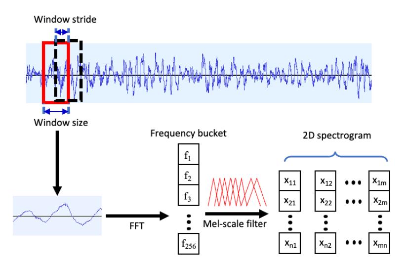
Deploying the trained ML models on small MCUs or edge devices is becoming increasingly common. The regular input of a tinyML model is a 2D spectrogram image of 1D data that is proposed in this paper to create a fully customized function. A spectrum image generation algorithm is proposed to provide a solution for preprocessing data into 2D spectrum images for TinyML models. The algorithm of this function is also detailed for use in future works.
A spectrogram image generation function has been integrated into the TensorFlow Lite library. The function is fixed for sample applications of this library and is hard to customize for new applications. Based on deeply analyzing the built-in functions, a modified function is proposed by the authors. The principle of imaging is explained in [16]. Figure 3 shows the mechanism for creating 2D spectrogram images with x dimensions. To create each column, a sliding window runs along the signal, forming a data slice, the number of slices being the number of columns. These slices of data are FFT-transformed to produce an array containing 256 frequency buckets, each with a value between 0 and 255. These frequency buckets can be averaged together to produce a smaller number of frequency groups, forming rows.
Based on the procedure described in Figure 3, the algorithm to create a 2D spectrogram image with x dimensions from stored samples is displayed in Algorithm 4. The input, x[n], is the signal to draw the spectrogram image, and y[n] is the one-dimensional array containing the flattened spectrogram. SampleRate is the sampling rate of the signal. WindowSize is the size of the sliding window that slides along the signal to get each piece of the signal, and WindowStride is the distance of each sliding of the WindowSize, both measured in milliseconds. SliceCount is the number of window frames obtained by moving a window of size WindowSize by amount WindowStride, and SliceSize is the number of frequency intervals after the spectrogram is drawn. These are the sizes of 2D spectrogram image created with SliceCount as and SliceSize as in x dimensions.
Generation spectrogram procedure.
The characters a, b, c, d, and e are user input parameters that provide values for the SampleRate, WindowSize, WindowStride, SliceCount, and SliceSize variables, respectively. Data_sample_size is the number of samples of the sliding window converted from milliseconds according to Eq. (19):
\[Data\_sample\_size = WindowSize * SampleRate/1000\] (19)
Data_sample is an array containing the data of the sliding window. New_slice_data is an array containing data that has been converted to a spectrogram from the data of the sliding window. When the program is activated, the loop will be repeated for the number of times corresponding to the SliceCount value. During each iteration, the sliding window extracts an amount of data from the x[n] array corresponding to the size of Data_sample_size and converts it to a spectrogram by the GenerateMicroFeatures() function, a built-in function of the TensorFlow Lite library.
Algorithm 4: Spectrogram image generation.
Input : x[n]
Output : y[n]
SampleRate←a;
WindowSize←b;
WindowStride←c;
SliceCount←d;
SliceSize←e;
Data_sample_size←WindowSize* SampleRate/1000;
Data_sample[Data_sample_size];
new_slice_data[SliceSize];
new_slice←0;
slice_start←0;
slice_sample←0;
i←0;
j←0;
while new_slice< SliceCount do
      slice_start=new_slice* WindowStride
      slice_samples=slice_start*(SampleRate/1000);
      while i< Data_sample_size do
           Data_sample[i] = x[i + slice_samples];
           i=i+1;
      end
      new_slice_data = GenerateMicroFeatures(Data_sample, Data_sample_size, SliceSize);
      While j < Data_sample_size do
           y[j + slice_samples] = new_slice_data[j];
      end
      new_slice=new_slice+1;
end
return y;
The result is returned to the new_slice_data array, which includes the value of the frequency group SliceSize. Then, the data of the new_slice_data array is copied and the output array y[n]. This will be repeated SliceCount times to get SliceCount x SliceSize elements of an array y[n], which is equivalent to an image with SliceCount x SliceSize size. The GenerateMicroFeatures() function was modified to enable image parameters that can be fully customized. So, although Algorithm 4 is based on built-in functions of the TensorFlow Lite library, it can be used independently with the original framework. This could not be done with the original function.
Results and Discussions
Relationship between Sampling Rate and the Quality of Acquired Digital Data
The FFT was applied to the recorded data to analyze frequency components and compare the main frequency components of the data with the original signals. The outcomes indicate that the recorded data could well represent the actual signals, whose main frequency components are close together. However, the frequency error, which is the difference between the digital data and the actual signal, was proportional to the signal's frequency and independent of the sampling rate, as presented in Figure 4. The maximum error was 79.6 Hz (0.38%), occurring due to sampling the 20 kHz sine wave at 96 kHz. This indicates that the ADC module combined with the I2S module can be used to collect high-frequency signals more effectively.
The FFT analysis results of the signal obtained (blue lines) from ESP32 using MATLAB are shown in Figure 5. This figure shows that many additional frequency components appear on both sides of the main component. These frequencies have less power than the main signals frequencies. They should be the harmonics and noise created during sampling of the signal. These components should be filtered by digital filters to enhance the quality of the digital data. Figure 5 also depicts the frequency domain of the filtered data (red lines). The harmonics and noise have been effectively eliminated by digital filtering. It is clear that the additional frequency components have been filtered effectively. The sample digital data of a 1-kHz sine wave was sampled at 44.1 kHz and 96 kHz in the time domain, as indicated in Figure 6, where the generated noises clearly appeared in the digital data. After applying the digital filters, this noise was removed, and the amplitude of the filtered signal was slightly reduced compared to the original data. The filtered signal obviously became smoother because the harmonics and noise at high frequencies had been eliminated, as shown in Figure 5. This demonstrates the effectiveness of digital filters in data pre-processing and their applicability to embedded systems.
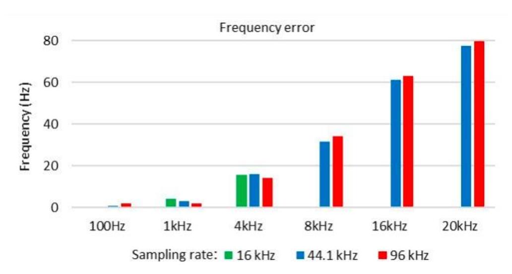
The error frequency of digital data at different sampling rates.
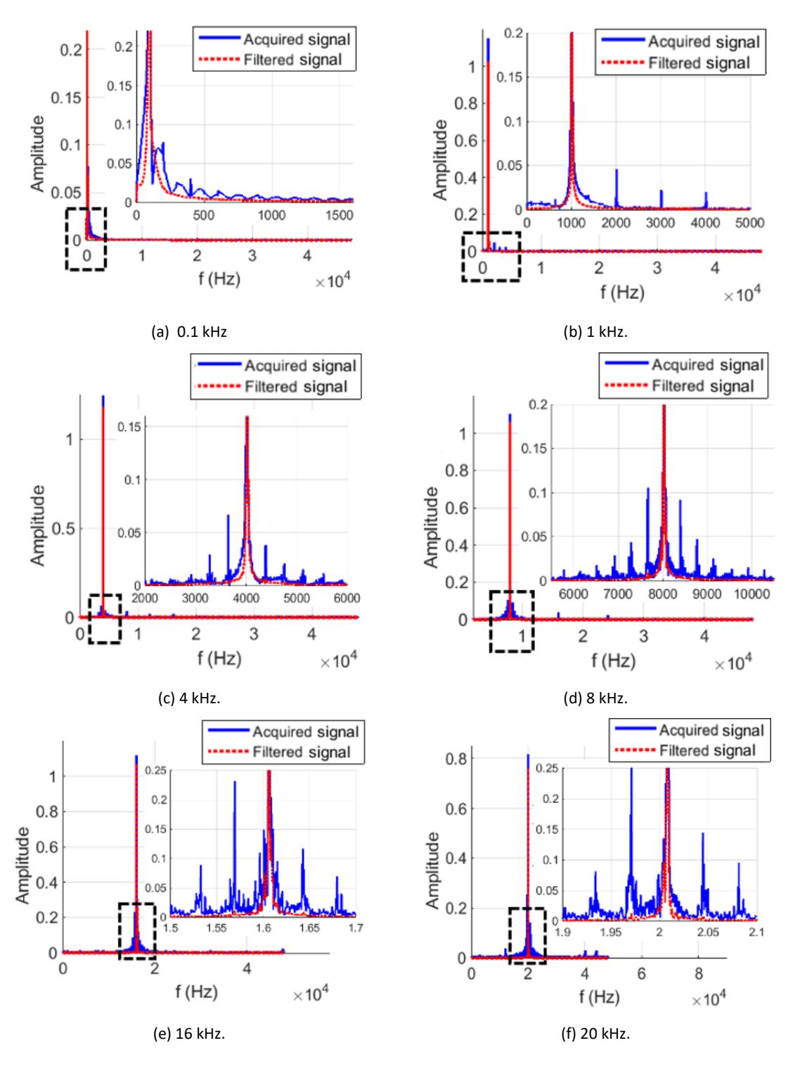
The FFT results of digital data sampling at 96 kHz, before and after applying digital filters.
The executive time of the filters is also a crucial aspect since they are intended to be deployed on resourcelimited MCUs. They have been coded and tested on an ESP32 MCU to measure their performance. Table 2 shows the filters' execution time to filter a signal consisting of 16,000 samples. These signals were collected at three sampling rates: 16 kHz, 44.1 kHz, and 96 kHz. The experimental results shown in Table 2 indicate that all filters were executed very fast, about 6.0 to 6.8 ms, to finish all calculations for filtering the 16,000 data samples. This indicates that the filter can run in real-time without significantly losing system processing time. This promises that it is possible to utilize them on embedded systems.
44.1
96.0
| Commis rote (kill=) | Filter type | ||
|---|---|---|---|
| Sample rate (kHz) | Low pass | High pass | Band pass |
| 16.0 | 6.83 | 6.83 | 5.97 |
6.83
6.83
6.85
6.84
5.99
5.98
Table 2 The execution time (ms) of the digital filters at different sampling rates.
In summary, when streaming converted data from the I2S module, the ADC module of the ESP32 MCU can acquire the analog signals efficiently. The digital data well represent the physical signals. Some harmonics and noise will be created, but these can be filtered out by the digital filters. The frequency error is proportional to the frequency of the signal, but it is only 79.6 Hz, equivalent to 0.38%, when acquiring a 20-kHz signal at a sampling rate of 96 kHz. These results prove that the ADC module of ESP32 should be combined with the I2S module to apply the DAQ for embedded applications.
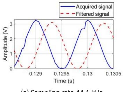
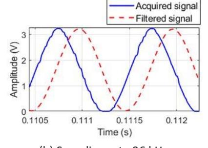
(a) Sampling rate 44.1 kHz.
(b) Sampling rate 96 kHz.
Figure 6 Results of filtering a 1-kHz sine signal with two different sampling rates using ESP32.
Table 3 shows the method comparison between this study and related studies. The comparative issues include the type of microcontroller, data acquisition module, maximum sampling rate, signal analysis and filters, and the type of signal used.
Table 3 Comparison of methods between this study and related studies.
| Study | Micro-controller board and Acquiring method | Maximum sampling rate (kHz) | Frequency error analyzing | Type of signal |
|---|---|---|---|---|
| Mobaraki et al. [5] | Arduino Mega, I2C protocol | None | None | Temperature |
| Babiuch et al. [6] | Various ESP32 Wrover, ADC | None | None | Sine wave and temperature |
| González et al. [8] | Arduino Due, SPI protocol and ADC | 2.56 | Yes (MATLAB tools) | Acceleration |
| Miquel et al. [10] | STM32L476, pulse-density modulation | 32 | Yes (decimation filter) | Audio |
| This study | ESP32-WROOM-32, I2S stream data | 96 | Yes (low-pass, high-pass, and band-pass filter) | Sine wave and white noise |
Spectrum Image Generation
The spectrogram image samples of the recorded data created by Algorithm 4 are shown in Figure 7 and 8. Figure 7 presents 35x35 spectrogram images generated directly on the MCU side using the modified function. The width is the time axis corresponding to the time of the original signal, and the height consists of frequency components of digital data from 0 to the sampling frequency. The magnitude of the frequency after distribution is in the range of an int8 data type [-128; 127]. The frequency of the sampled data is indicated by the location line pointed out by the red arrows. At the frequency position of the signal, the brightness of the pixel is higher than the rest of the image. The image clearly shows the frequency position of the signal and can be recognized with the naked eye.
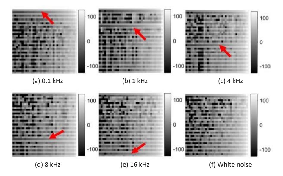
Amplitude spectrograms of recorded data with noise reduction.
Figure 8 also shows the spectrogram images of the same data as in Figure 7, but the noise reduction algorithm of the original function is ignored. In these spectrogram images, the frequency components are shown over time, apparently. The main frequency component of the data is also a line, as indicated by the red arrows, and is clearer than in Figure 7. The difference in the frequency distribution is very obvious. The original frequency region of the sine signal is brighter than the other regions. Meanwhile, the spectrogram image of white noise has a uniform brightness distribution because white noise is composed of sine waves of all frequencies. Both types of images simultaneously show the time and frequency domains of the acquired data. They have been used as input for tinyML models in recognition and classification applications on MCUs. The ESP32 MCU only takes 40 ms to create one spectrogram image. The spectrogram generation time includes 35 FFT transforms for each data segment, so the time of one FFT transform is approximately 1.14 ms, which is reasonable to use for real-time applications.
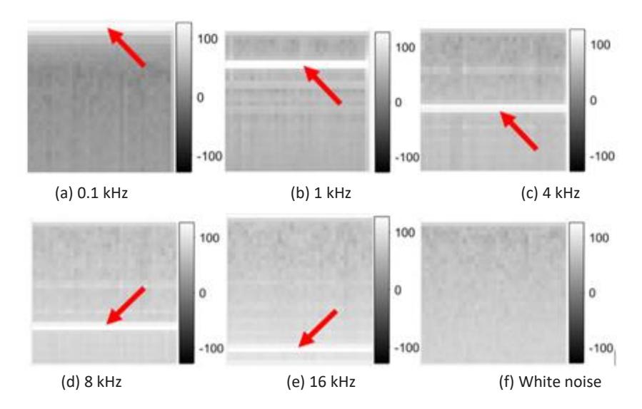
Amplitude spectrograms of recorded data without noise reduction.
Discussion
This study proved that the ADC module on the ESP32 MCU can be used to acquire data, except that its data should be streamed by the I2S module. The experimental results show that the frequency error is only
proportional to the signal frequency and up to 79.6 Hz at a sampling rate of 96 kHz, equivalent to 0.38%. This means that the higher the frequency of the original signal, the larger the error of the collected signal. The frequency error of the collected data is proportional to the frequency of the signal and independent of the sampling rate. Therefore, a sampling rate of 96 Khz is suitable for collecting high-frequency data when using the proposed feature. The 4th-order Butterworth low-pass and high-pass filter, and the second-order band-pass filter have been productively deployed on the ESP32 to filter the digital data. The execution times of these filters were fast and less than 7 ms. In addition, a customized function to create the spectrogram image was provided, which could successfully generate two types of images directly from the sampled data. The time required to create a spectrogram was only 40 ms. The function is ready to be used for processing data to run tinyML models on MCUs, especially the ESP32 MCU.
Some remaining issues should be considered. Firstly, the FFT results revealed that harmonics and noise are created in the recorded data beside the main frequency component. The digital filters could eliminate them to enhance the quality of the digital data. However, the results only showed single sine wave data; the digital filters should be applied to the real signal in some specific applications to evaluate their effectiveness. Next, the frequency of high-speed physical signals is not sampled accurately, with a small remaining error. A suitable solution should be proposed to reduce this error. Last but not least, the I2S module is not integrated in many MCUs and therefore improving the sampling speed of the ADC module should be considered to enhance the quality of the sampling data in embedded applications.
Conclusion
This study proposed a data acquisition system that applied the ADC and I2S modules of the ESP32 to acquire high-frequency data. The ADC module of the ESP32 showed good performance in the DAQ when combined with the I2S module. The experiments showed that the error of the received signal was proportional to the frequency of the original signal. The sampling rate does not affect the accuracy of the collected data when the Nyquyst theorem is followed. Therefore, a sampling rate of 96 kHz is suitable for collecting high-frequency data when using the proposed feature. In addition, the proposed digital filters have extremely fast execution times and therefore can be used in real-time applications on embedded systems. The test results showed that the filters effectively removed the noise from the received signal. Furthermore, a spectrum image generation algorithm was developed to convert the data into images in the frequency domain. This feature can be applied to preprocess data into 2D spectrogram inputs for TinyML networks on embedded systems.
This study had some limitations that need to be addressed. For instance, the experiment needs to be extended to more complex data types to evaluate the data collection ability of the proposed feature. In addition, digital filters cannot remove noise that appears immediately next to the original signal. Finally, the I2S module is not integrated into many MCUs. Therefore, implementing the proposed features on another microcontroller family should be considered to avoid affecting data quality. In the future, more complex data filtering algorithms, such as FFT-based or wavelet transform-based filters, will be researched. Moreover, we will focus on implementing TinyML models based on the proposed features.
Compliance with ethics guidelines
The authors declare that they have no conflict of interest or financial conflicts to disclose.
This article does not contain any studies with human or animal subjects performed by any of the authors.