
Introduction
Wet flue gas desulfurization (WFGD) absorbers are commonly used to remove SO2 emitted from CFPPs. Limestone is widely applied as an absorbent, since it is simple, cheap and was the most developed SO2 wet removal process available from the early 1980s until the 1990s. However, the use of limestone still carries some inherent challenges such as mining source availability, transportation to the CFPP site as well as byproducts (gypsum) management. Although gypsum has an economic value, it is classified as a hazardous material in Indonesia according to the Government of Indonesia Regulation No. 101/2014 concerning Waste Management of Hazardous and Toxic Materials. Thus, gypsum from WFGD absorber byproducts must be handled as a hazardous material, which eventually leads to an increase of the operational cost of CFPPs.
Based on data from three major international SWFGD vendors, SWFGD processes have been used since 1995 but gained attention and popularity from 2010. At least two seaside CFPPs in Indonesia applied this system in 2019. There are two main advantages of utilizing seawater as absorbent, i.e., the abundant availability of absorbent, especially in a maritime country such as Indonesia, and simple effluent handling due to the absence of unwanted byproducts [1]. The salinity of seawater used is highly dependent on the region and the conditions of the waters under consideration, but the cation and anion constituents contained in the water are approximately the same. Alkali compounds generally present in seawater are HCO3 - , CO3 2- , OH- , HPO4 2- and other trace elements. The main contributor to the alkalinity of seawater is HCO3- [1], and the common seawater salinity is 35 ppt (g/kg) [2]. Table 1 summarizes the differences between a WFGD and an SWFGD.
Parameter WFGD SWFGD Source SO2 removal efficiency 80 – 95% 95 – 99% 90 – 98% 90 – 95% [3] [4] pH – Inlet – Outlet 4.73 – 6.59 8.0 – 8.2 3.0 – 4.0 [3] [5,3] Generated byproduct Large amount of gypsum - [3] Effluent characteristics Increased Slight increase [3]
Table 1 Differences in SO2 removal efficiency, pH and generated byproduct of a WFGD and an SWFGD absorber.
After being used as an absorbent in removing SO2 gas in an SWFGD absorber, the seawater pH in the SWFGD absorber effluent will decrease due to the increase of acid species. Therefore, it must be treated using aeration before being released back to the sea and mixed with additional seawater from the condenser. During aeration, large amounts of oxygen (O2) gas will be injected to remove dissolved CO2 in the water [6] and oxidize SO3 2 to SO4 2 to reduce chemical oxygen demand (COD) [3].
suspended solids of SO4 2-
A numerical study that modelled the interface between seawater and SO2 gas in a single droplet of seawater for maritime engines has shown that seawater can be used as a promising absorbent compared to conventional ones such as NaOH, limestone, and NaCl [1]. Another numerical study was carried out in a maritime engine, considering salinity as the limiting factor in the chemical reaction [2]. Similar numerical modelling, which correlated the equilibrium constant of the absorption process and the removal efficiency of SO2 within a packed tower, was done previously [7].
The present study combined the numerical model results given by [7] and [2] as well as other modelling information from [3, 6, 8, 9, 10-17], which was then used to evaluate the applicability of seawater in a flue gas desulfurization process in Indonesia.
Methodology
A model was set up based on the reaction balance, mass balance, and energy balance of SO2 absorption within an SWFGD absorber. Results of the calculations are presented in the form of SO2 concentration and temperature along the SWFGD absorber. A typical system of an SWFGD absorber (a packed tower type) is illustrated in Figure 1. The changes in concentration or mole faction of the SO2 in the gas stream along the height of the absorption tower are illustrated in Figure 2.
An SWFGD system with an aeration tank.
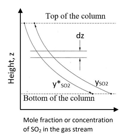
Figure 2 Simplified schematic diagram of the changes in SO<sub>2</sub> mole fraction in the absorption tower [18].
The absorption tower operates in a counterflow configuration with liquid flowing down the column by gravity and the gas flowing up the column driven by the decrease in pressure from bottom to top. The curve in Figure 2 shows that the mole fraction of \(SO_2\) (\(y_{SO2}\)), the gas to be absorbed, decreases from its high value where it enters the bottom of the absorption tower to its low value at the outlet of the absorption tower. The curve also shows the mole fraction of \(SO_2\) (\(y^*_{SO2}\)) that would be in equilibrium with the liquid absorbent, its value increasing from the top of the column to the bottom of the column, as absorbent removes the \(SO_2\) from the gas stream.
Model Assumptions
The SO<sub>2</sub> absorption model in seawater absorbent used in this study is a non-isothermal model considering chemical reactions in the gas and liquid phases. The mass balance, the coefficient of heat transfer resistance in the gas and liquid phases and the evaporation of the liquid form the basis for the preparation of mathematical models. The model was developed for the steady state adiabatic operating conditions with fluctuations in gas and liquid discharge due to evaporation with resistance due to heat transfer not being taken into account.
Henry's Law and Dissociation-Neutralization Reaction
The following sequence of chemical reactions shows the absorption of \(SO_2\) from gas phase to liquid phase in Eq. (1), bisulfite \(HSO_3^-(aq)\) in Eq. (2), dissociation reaction of bisulfite to sulfite \(SO_3^{2-}(aq)\) in Eq. (3), neutralization of \(H_3O^+(aq)\) that has been formed by the seawater in Eq. (4), dissociation reaction of hydrogen sulfate to sulfate present in the seawater in Eq. (5), absorption of \(CO_2\) gas in water in Eq. (6), the dissociation of water into \(H^+\) and \(OH^-\) in Eq. (7).
\[SO_2(g) \leftrightarrow SO_2(aq)\] (1)
\[SO_2(aq) + 2H_2O(l) \leftrightarrow HSO_3^-(aq) + H_3O^+(aq)\] (2)
\[HSO_3^-(aq) + H_2O(l) \leftrightarrow SO_3^{2-}(aq) + H_3O^+(aq)\] (3)
\[HCO_3^-(aq) + H_3O^+(aq) \leftrightarrow CO_2(aq) + 2H_2O(l)\] (4)
\[HSO_4^-(aq) + H_2O(l) \leftrightarrow SO_4^{2-}(aq) + H_3O^+(aq)\] (5)
\[CO_2(aq) \leftrightarrow CO_2(g)\] (6)
\[H_2O \leftrightarrow H^+ + OH^- \tag{7}\]
The dissolution reaction of \(SO_2\) in the gas phase into the water phase occurs in a thin film layer that separates the gas and water according to Henry's law in Eq. (8):
\[[SO_2(aq)] = p_{SO_2}k_H \tag{8}\]
Where \(pSO_2\) is the partial pressure of \(SO_2\), \([SO_2(aq)]\) is the concentration of \(SO_2\) in the solution and \(k_H\) is Henry's constant expressed by Eq. (9):
\[k_H = k_H^{\circ} e^{\frac{-\Delta H_{Soln}}{R} (\frac{1}{T} - \frac{1}{T^{\circ}})}\] (9)
Where k°H is Henry's constant under reference conditions, Hsoln is the enthalpy of the solution, T is the temperature and T° is the temperature at the reference condition (298.15 K). By entering Henry's constant obtained from experiment [15], a value for kH° value of 1.2 mole/(kg atm) was derived with a slope (-Hsoln/R) of 2850 K. This was in accordance with the data listed in [19]. Calculation of chemical compound changes in the system is a function of the temperature-dependent dissociation coefficient. The dissociation coefficient developed in [10] has a limited seawater temperature range of 278.15 to 318.15 K. In this case, the dissociation coefficient calibration was applied based on temperature differences [20]. Dissociation coefficient calibration is shown in Eq. (10).
\[ln\frac{K_{(T_2)}}{K_{(T_1)}} = \frac{-\Delta H^{\circ}}{R} \left(\frac{T_1 - T_2}{T_1 T_2}\right) \tag{10}\]
The dissolution and neutralization processes in reaction 2 to 5 can be expressed by Eqs. (11) to (14):
\[K_{II} = \frac{[HSO_3^-][H_3O^+]}{[SO_2(aq)]} \tag{11}\]
\[K_{III} = \frac{[so_3^{2-}][H_3o^+]}{[HSO_3^-]} \tag{12}\]
\[K_{IV} = \frac{[CO_2(aq)]}{[HCO_3^-][H_3O^+]} = K_a^{-1}\] (13)
\[K_V = \frac{[SO_4^{2-}][H_3O^+]}{[HSO_4^-]} \tag{14}\]
Salinity is another factor that has an influence on the constant Ka. The empirical correlation between temperature and salinity is described in Eq. [11], where S is the salinity and A, B, C, D, and E are coefficients that depend on temperature as expressed in Eqs. (15) and (16):
\[\ln K_a = A + BS^{0,5} + CS + DS^{1,5} + ES^2 \tag{15}\]
\[\operatorname{Ln} K_* = 2,83655 - \frac{2307,1266}{T} - 1,4429413 \ln T + \left(-0,20760841 - \frac{4,0484}{T}\right) S^{0,5} + 0,08468345S - 0,00654208S^1\] (16)
Mass Balance
Mass balance and energy balance equations were derived from [7]. The size of the WFGD can be determined by applying the principle of mass transfer as in Eq. (17):
\[ln\frac{y_{out}}{y_{in}} = K_g a \frac{P}{G^1} \tag{17}\]
Where yin is the SO2 concentration at the inlet (ppm), yout is the SO2 concentration at the outlet, Kg is the overall mass transfer coefficient (kg mole/m2 hour atm), P is the pressure (atm), a is the gas-liquid contact area (m2 /m3 ), and G1 is the molear mass velocity of the gas (kg mole/m2 hr).
The global mass transfer coefficient can be determined using Eq. (18):
\[\frac{1}{K_g} = \frac{1}{k_g} + \frac{H}{\emptyset k_L} \tag{18}\] where kg is the mass transfer coefficient of the gas phase (kg mole/ m2hour atm), kL is the mass transfer coefficient of the liquid phase (m/hour), H is Henry's constant for SO2 (atm hour/kg mole), and Φ is the enhancement factor. The values of kg and kL were taken for packed towers of the Raschig rings type [17].
The variation of SO2 concentration in the gas phase along the absorber can be described by Eq. (19):
\[\frac{dy_{SO_2}}{dz} = -\frac{N_{SO_2}AaM_a}{Q_g\rho_g} \tag{19}\] with the mass transfer flux (NSO2) derived from Eq. (20):
\[N_{SO_2} = K_{gs}(y_{SO_2} - y_{SO_{2i}}) (20)\]
In the above equation, ySO2i is the equilibrium concentration of SO2 in the gas phase, and Kgs is the overall mass transfer coefficient of SO2, which is calculated based on the mass transfer coefficients of the gas and liquid phases.
The calculation of the SO2 fraction (ySO2i) at equilibrium condition is estimated using Eqs. (21) and (22):
\[\{H^{+}\} = \frac{10^{-pH}}{\gamma_{H^{+}}} + [HSO_{3}^{-}] + 2[SO_{3}^{2-}] - [H_{2}CO_{3}^{*}]_{g} - [HSO_{4}^{-}]\] (21)
where [H2CO3*]g represents the H2CO3 and CO2(aq) species during the SO2 absorption process with [H2CO3*]g = [H2CO3*]i - [H2CO3*]f. The subscripts g, i and f refer to the gas, interface, and fluid in respective order. As a simplification, the value of [H2CO3]f = CO2(aq) because it is dominated by CO2(aq) species. The concentration of [H2CO3]i in water is the HCO3- species produced by the reaction of CO2(aq) with water [9]. The initial alkalinity of seawater, which is 2400 mole/kg H2O, is also added as initial condition.
\[y_{SO_{2i(aq)}} = \frac{T_{SO_2} x H_{SO_2}}{P} \left[ \frac{1}{\gamma_{SO_2}} + \frac{K_{II}}{\{H^+\} x \gamma_{HSO_3}} + \frac{K_{II} x K_{III}}{\{H^+\}^2 x \gamma_{SO_3}} \right]^{-1}\](22)
For every variation of SO2 concentration along the absorber, there is an equilibrium in both phases as a function of temperature, partial pressure of SO2 in the gas phase, and the composition of seawater. The variation of water vapor in the gas phase along the absorber is described by Eq. (23):
\[\frac{dy_w}{dz} = \frac{N_w A a M_a}{Q_g \rho_g} \tag{23}\] with the mass transfer flux described by the notation Nw as in Eq. (24):
\[N_{w} = k_{gw}(y_{wi} - y_{w}) \tag{24}\]
The concentration of SO2 gas passing through the gas layer will be absorbed in the liquid according to the Two-Film Theory law with the mass balance equation for the SO2 gas concentration in the liquid phase (Xd) along absorber described by Eq. (25):
\[\frac{dX_d}{dz} = -\frac{N_{SO_2}AaM_W}{Q_l\rho_l} \tag{25}\]
Energy Balance
The transfer of water vapor from the liquid layer to the gas layer occurs due to the simultaneous transfer of mass and energy. The variation in temperature (energy balance) of the gas phase along the absorber is described by Eq. (26):
\[\frac{dT_g}{dz} = -\frac{haA(T_g - T_l)}{Q_g \rho_g (C_{pg} + y_w C_{pv})} \tag{26}\]
The liquid temperature depends on the convection coefficient of the gas, the evaporation of the liquid, and the heat generated from the reaction. The variation in temperature (energy balance) of the liquid phase along a point in the absorber is described by Eq. (27):
\[\frac{dT_l}{dz} = -\frac{N_w a A M_w \gamma + h a A (T_g - T_l) + \Delta H_r N_{SO_2} M_{SO_2}}{Q_l \rho_l C_{pl}}\] \[(27)\]
Solution of Numerical Model
Figure 3 illustrates the schematic of numerical model solution. Gin and Gout refer to the direction of gas flow, whereas Lin and Lout refer to the direction of liquid flow. Gas and liquid come in contact in a counter current motion. Temperature undergoes a change throughout the tower (Figure 3 – left). Parameters such as temperature, pH and SO2 removal efficiency are determined at certain heights of the tower denoted by cell i and j (Figure 3 – middle). The model is solved using an explicit finite difference method (4th -order Runge-Kutta), where the output of the previous calculation step (e.g. cell i) is used as input to find the solution of the next step (e.g. cell i + 1) (Figure 3 – right). Corresponding equations as described in Eq. (8) to (27) were solved numerically with the schematic numerical model solution illustrated in Figure 3.
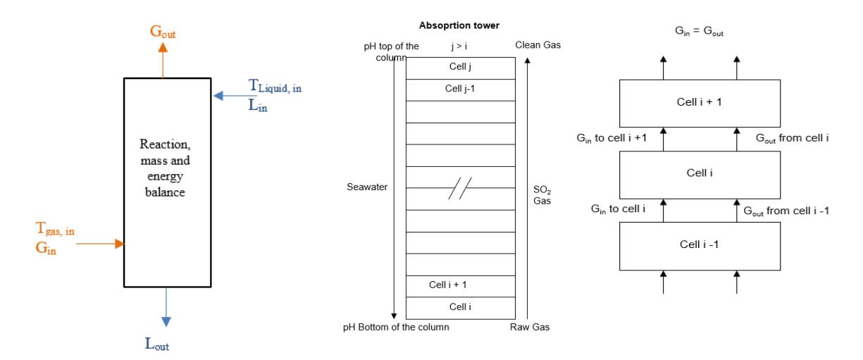
Figure 3 Schematic of numerical model solution in an absorption tower.
Results and Discussion
This study used field-scale data from an SWFGD absorber located in West Java, Indonesia. Model running was done by using a Henry's constant derived from said reference and additional information such as SWFGD dimension, flue gas temperature, seawater temperature, and both gas (1,691,277 Nm³/h) and liquid (68,912 m³/h) flowrate.
Chemical Species in Seawater
Table 2 shows the corresponding sulfur containing chemical species present in the seawater along the absorption tower. A general trend of the decrease of mole fraction of \(SO_2\), \(SO_3^{2-}\), \(SO_4^{2-}\), \(HSO_3^{-}\) can be observed, as the distance from the bottom of the tower increases. On the other hand, an \(HSO_4^{-}\) increase can be observed, as the distance from bottom tower increases. If correlated with the corresponding pH, at a final pH of around 4.19, the seawater composition was dominated by \(HSO_3^{-}\).
| Distance form | Species concentration (mole/kg) | |||||
|---|---|---|---|---|---|---|
| bottom tower (m) | SO2 | SO32- | SO42- | HSO₃- | HSO4- | |
| 0.00 | ||||||
| 0.25 | 5.799668 | 0.157513 | 0.005485 | 155.0613 | 8.92E-06 | |
| 2.75 | 5.527831 | 0.127626 | 0.005484 | 143.1394 | 9.28E-06 | |
| 5.25 | 5.230671 | 0.115468 | 0.005484 | 130.5496 | 9.72E-06 | |
| 7.75 | 4.903825 | 0.075943 | 0.005483 | 117.2456 | 1.03E-05 | |
| 10.25 | 4.541677 | 0.051641 | 0.005483 | 103.1836 | 1.09E-05 | |
| 12.75 | 4.136818 | 0.016279 | 0.005482 | 88.32917 | 1.18E-05 | |
| 15.25 | 3.680244 | 5.20E-07 | 0.005481 | 72.70805 | 1.30E-05 | |
| 17.75 | 3.149669 | 4.67E-07 | 0.005479 | 56.11986 | 1.48E-05 | |
| 20.25 | 2.517221 | 4.54E-07 | 0.005476 | 38.66107 | 1.79E-05 | |
| 22.75 | 1.666776 | 4.23E-07 | 0.005469 | 19.48326 | 2.52E-05 | |
| 25.00 | 0.857215 | 4.17E-07 | 0.005450 | 6.426894 | 4.39E-05 | |
Table 2 Chemical species in seawater.
Ph Value and Corresponding SO<sub>2</sub> Concentration in Gas Phase
Figure 4 shows the simulation result of the pH value along the absorption tower. By using an initial pH of 7.5, the final pH at the bottom of the tower was predicted to be 4.19. An abrupt decrease of pH at 22.75 m from the bottom of the tower was caused by the amount of \(SO_2\) absorbed in the seawater, i.e., 5.79 mole/kg or 0.09 g/kg, close to the calculation result in [2].
Figures 5 and 6 show the removal efficiency of \(SO_2\) concentration in the SWFGD absorber. Removal efficiency refers to the absorption of \(SO_2\) from gas to liquid phase in seawater. At the farthest point from the bottom of the tower, removal efficiency reached 30.6% with a corresponding \(SO_2\) concentration of 208.5 ppm. Comparison of data with the existing flue gas desulfurization absorber in an actual scale with the similar gas and liquid flowrate, the pH and initial \(SO_2\) concentration resulted in a removal efficiency of 32.9% based on the SWFGD study in Indonesia.

Figure 4 Value of pH along the absorption tower.
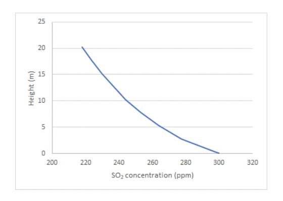
Figure 5 SO<sub>2</sub> concentration in the SWFGD absorber.
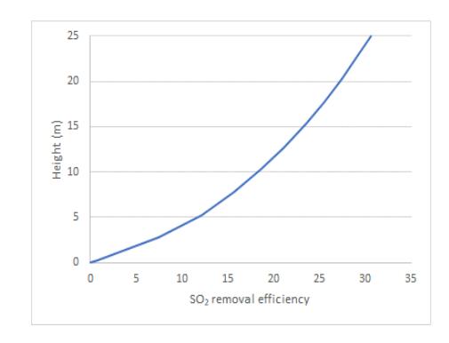
Figure 6 \(\,\) SO\(_2\) removal efficiency in the SWFGD absorber.
Temperature
Figures 7 and 8 show the simulation result of the gas and liquid temperature along the counter current SWFGD absorber in the form of a percentage of the temperature decrease. As the mixing of the gas and liquid phase occurs simultaneously, it is obvious that the gas temperature will decrease from the bottom to the top of the tower (the gas is injected from the bottom of the tower), and the liquid temperature will increase from the top to the bottom of the tower (the liquid is injected from the top of the tower).
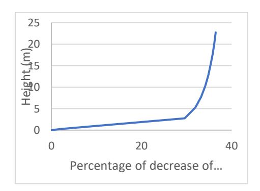
Figure 7 Percentage of decrease of the seawater temperature in the SWFGD absorber.
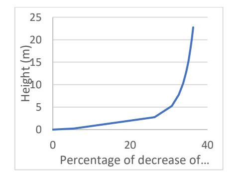
Figure 8 Percentage of decrease of the gas temperature in the SWFGD absorber.
Additional Model Testing (Mass Transfer Coefficient)
Table 3 shows the result of overall mass transfer coefficient testing with a kl value of 0.083/s and 0.0415/s, respectively. With a lower overall mass transfer coefficient, a lower removal efficiency is produced. The result of overall mass transfer coefficient calibration is in accordance with the removal mechanism in a flue gas desulfurization absorber, where the increase of the overall mass transfer coefficient in the liquid phase will lead to a higher amount of SO2 absorbed in the liquid. In this case, the decrease of the overall mass transfer coefficient in the liquid phase lowered the removal efficiency by 12.27% point. This value is very high relative to the initial removal efficiency.
| Concentration (fraction) | Efficiency (%) | |||
|---|---|---|---|---|
| Distance from bottom tower (m) | kl1 | kl2 | kl1 | kl2 |
| 0.00 | 0.000300 | 0.000299 | 0.000000 | 0.000000 |
| 0.25 | 0.000298 | 0.000297 | 0.760574 | 0.496849 |
| 2.75 | 0.000277 | 0.000285 | 7.509737 | 4.692743 |
| 5.25 | 0.000264 | 0.000277 | 12.1268 | 7.403493 |
| 7.75 | 0.000253 | 0.000271 | 15.6785 | 9.470021 |
| 10.25 | 0.000244 | 0.000266 | 18.63664 | 11.19566 |
| 12.75 | 0.000236 | 0.000261 | 21.19987 | 12.70009 |
| 15.25 | 0.00023 | 0.000257 | 23.47766 | 14.04719 |
| 17.75 | 0.000223 | 0.000254 | 25.53798 | 15.27565 |
| 20.25 | 0.000218 | 0.000250 | 27.42626 | 16.41100 |
| 22.75 | 0.000212 | 0.000247 | 29.17442 | 17.47101 |
| 25.00 | 0.000208 | 0.000245 | 30.64737 | 18.37134 |
Table 3 Overall mass transfer coefficient calibration (kl1 = 0.083 and kl2 = 0.0415).
Additional Model Testing (Laboratory-scale Experiments)
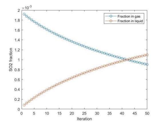
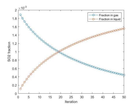
Due to limited field data, additional testing with laboratory-scale experiments was carried out to determine the model's validity. The parameters, i.e., packing details, salinity, pH, gas and liquid flowrate, L/G ratio and SO2 concentration, were derived from [21] and were run using the same algorithm as previously presented. Figures 9 and 10 show the simulation results with SO2 concentration being held constant at 500 ppm. The liquid flowrate was run at 40 L/h and 130 L/h, which corresponds to an L/G ratio of 1.06 kg/kg and 3.44 kg/kg, respectively. The developed model was found to be sensitive towards the increase of the L/G parameter with higher efficiencies present for a higher L/G value.
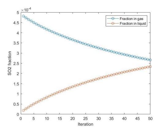
SO2 fraction (initial SO2 concentration = 500 ppm and L/G 1.06 kg/kg).
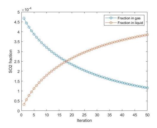
SO2 fraction (initial SO2 concentration = 500 ppm and L/G 3.44 kg/kg).
Moreover, the simulation results with the SO2 concentration being held constant at 2,000 ppm (which corresponds to the highest concentration reported in [21]) produced a similar trend. Figures 11 and 12 show the simulation result with the SO2 concentration being held constant at 2,000 ppm. The liquid flowrate was run at 40 L/h and 130 L/h, which corresponds to an L/G ratio of 1.06 kg/kg and 3.44 kg/kg, respectively. A reduction in removal efficiency is to be expected, since the SO2 concentration is increased with the L/G ratio being held constant. Table 4 summarizes a comparison between the SO2 removal efficiency reported in [21] and the developed model.
SO2 fraction (initial SO2 concentration = 2000 ppm and L/G 1.06 kg/kg).
SO2 fraction (initial SO2 concentration = 2000 ppm and L/G 3.44 kg/kg).
Table 4 Comparison of SO2 removal efficiency.
| Parameter | Mass transfer coefficients (mole/m2s) | Efficiency (%) | ||
|---|---|---|---|---|
| Gas | Liquid | Model | Reference* | |
| 500 ppm | ||||
| L/G: 1.06 kg/kg | 0.8 | 2.5 | 46.8 | 64 |
| L/G: 3.44 kg/kg | 1 | 1 | 76.9 | 90 |
| 2000 ppm | ||||
| L/G: 1.06 kg/kg | 0.5 | 3 | 54.9 | 24 |
| L/G: 3.44 kg/kg | 0.8 | 4 | 77.8 | 72 |
*Reference is given as an estimate [21]
The discrepancies are likely caused by different assumptions of mass transfer coefficients used in the developed model. Additional running was done with a liquid and vapor mass transfer coefficient with a rate-based column of Sulzer MellaPak 250Y. The developed model showed adequate resemblance at a lower SO2 concentration but overestimated the removal efficiency at a higher concentration. The model is able to show the general trend of SO2 removal in an SWFGD, however refinement is needed to increase the model's accuracy. Although the developed model was proven to be sensitive towards variation of the liquid mass transfer coefficient (as shown in Table 3), further experimental-scale reactor testing is needed to validate the results.
Conclusion
Simulation of SO2 absorption in an SWFGD absorber was carried out utilizing field data input from an existing SWFGD absorber in Indonesia. Calculation results showed that the developed model was able to illustrate that the changes in SO2 concentration, pH as well as the removal efficiency along the absorption tower, were in accordance with the theory. The concentration distribution in SWFGD followed an exponential pattern, where a decrease of SO2 gas with increasing tower height was observed. Temperature would decrease with an increase of SWFGD absorber height. However, some discrepancies were found due to the lack of information on several constants for the mass transfer of seawater absorbent. Differences in results can be overcome by validating the model with experimental-scale reactor testing.
Acknowledgement
This research was carried out with the help of funding from Pengabdian kepada Masyarakat dan Inovasi ITB (P3MI) ITB in 2019.
Compliance with ethics guidelines
The authors declare that they have no conflict of interest or financial conflicts to disclose.
This article does not contain any studies of human or animal subjects performed by any of the authors.