
Introduction
In previous years, the lighting effectiveness of modern LEDs (light emitting diodes), particularly the GaN-based ones, has received considerable interest due to their exceptional qualities over traditional light sources, including extended life, environmental protection, and low consumption, etc. It is well known that the junction temperature TJ of multi-chip LED packages has a major impact on the reliability of LEDs. Approximately 70% of the electrical power entered into LEDs at their optimal current densities is currently converted to heat. High temperatures reduce the lifetime of LED chips and limit LED light production. LED chips are susceptible to catastrophic damage when the junction temperature exceeds 120℃[1, 2]. Many studies have examined the impacts of thermal and electrical stress on these components [3]. The topic of thermal management of LED packages has been investigated by several authors. Abdelmalek et al. [4] created models to evaluate LED package thermal behavior, which were verified with experiments. To improve heat performance, optimization techniques have been integrated into these models. Unfortunately, those authors' simulation methods were deterministic and did not take into account the variability of performance due to the uncertainty of the design parameters. To overcome this problem, this article offers the optimum design of LED packages with a high level of reliability. In our research, the thermal behavior of the model was first analyzed and modeled by Finite Element Method (FEM). The results were compared with the reference results [4, 5] to confirm our finite element model. When the purpose of study is to determine the main factors that affect the thermal behavior of a LED package and to find the best value for each factor, the sensitivity analysis method (SA) is a proven approach [6-11]. SA often includes both local and global sensitivity analyses (LSA and GSA). The global sensitivity analysis (GSA) method is an option to solve this problem. This solution consists of using a system capable of managing complicated situations in order to integrate the interactions between the input parameters and to reliably determine the distinct contributions of each variable. Naturally, a reliability study based on performance
Copyright ©2024 Published by IRCS - ITB J. Eng. Technol. Sci. Vol. 56, No. 4, 2024, 521-534 ISSN: 2337-5779 DOI: 10.5614/j.eng.technol.sci.2024.56.4.8
simulations should be carried out, which is even more important for engineering applications of LED lighting [12- 15].
To determine whether a specific design will meet specific performance or reliability needs, reliability assessment attempts to evaluate the reliability of LED lighting and identify the most important design parameters, as well as to provide useful information for design optimization and improvement. In this paper, the focus is on the mechanism, which is considered to be the weakest component of LED packages based on previous design experience. To decrease the computational constraints caused by recurrent performance function evaluations in reliability analysis, approximation approaches are utilized. We used Monte Carlo simulation (MCS), the most common method, which is categorized as a probabilistic approach. However, MCS requires an extended calculation period. The FORM/SORM methods are recommended probabilistic approaches to reduce computational constraints induced by the repeated evaluation of performance functions. Using this method, we may determine the sensitivity of the reliability index to the parameters of random variables. Nevertheless, the reliability analysis allows for the determination of the level of reliability or the probability of failure in relation to factors that lead to component failure. Additionally, there are methods that can be employed to raise the reliability level. Reliability-Based Design Optimization (RBDO) allows for increasing a structure's reliability at minimal cost [14-19]. To reduce the cost of computing, we proposed the Sequential Quadratic Programming (SQP) technique for RBDO problem-solving. RBDO approach aims to improve the design and achieve high reliability in comparison to the stated failure scenario.
Material and Methods
The Model of Multi-Led Chip Package
Geometry and Material Properties
The GaN (gallium nitride) LED was chosen asthe focus of thisresearch. We designed a model that was developed in [4, 5]. In this model, the Si-die and COB-LED chips are linked together by an Au-Si eutectic bond. The die is connected to an insulated substrate using a die-attach. The Au-20Sn is used to connect the Si-die to the insulated substrate. The LED chip is fixed in a heat sink using thermal grease (TIM). Figure 1(a) depicts the design of a multi-led chip package. As presented in Figure 1(b), the package consists of nine chips, with a pitch between two adjacent LEDs of 3 mm [4]. Table 1 displays the dimensions of various materials and the thermal characteristics of the model, where is thermal conductivity [20].
(a) Structure of the model and (b) the pitch refers to the space between LEDs.
| Table 1 | Dimensions and thermal conductivities of the LED package components. |
|---|
| Components | Thickness (µm) | Size (mm2 ) | Materials | (W/m.K) | |
|---|---|---|---|---|---|
| LED chip | 4 | 1.0×1.0 | Gallium nitride | 130.0 | |
| Die | 375 | 1.0×1.0 | Silicon | 124.0 | |
| Metallization | 10 | 1.0×1.0 | Au-Si Eutectic bonding | 27.0 | |
| Die-attach | 50 | 1.0×1.0 | Au-20Sn | 57.0 | |
| 127 | 1.0×1.0 | Copper | 385.0 | ||
| Substrate | 75 | 1.0×1.0 | Dielectric | 1.10 | |
| 1000 | 1.0×1.0 | Aluminum | 150.0 | ||
| TIM | 50 | 1.0×1.0 | Thermal grease | 3.0 | |
| Heat sink | Base | 2mm | 20.0×20.0 | Aluminum | 150.0 |
| Fin | 18mm | 1.50×20.0 | Aluminum | 150.0 | |
Assumptions and Boundary Conditions
For all cases, the ambient temperature, Tamb, of the whole model was set to 25 ℃. The top of each LED chip is supposed to receive a consistent heat flow of 3.5 W [4]. The thermal convection coefficient is h = 10 W/m2 .K. The ability of natural convection to remove heat from these components is essentially nonexistent due to the small surfaces involved [21, 22]. The heat transfer problem of the LED package was modeled using the following hypotheses:
- 1. The materials of the package are all homogenous, isotropic, and temperature-neutral.
- 2. Each layer of material is airspace-free.
- 3. Only heat dissipation during natural convection is considered.
Finite Element Modeling
Based on the above assumptions, the three-dimensional finite-element heat transfer model was chosen to investigate the thermal control performance of the system. The governing equations that were utilized to solve the numerical model are provided below. The local heat equation is a mathematical formula presented in Eq. (1) [23]:
\[\lambda \nabla \cdot (\nabla T) - \rho \dot{CT} = 0 \tag{1}\] where . is the divergence operator, is the gradient operator, and T is the temperature field (K).
As shown in Table 1, the dimensions and thermal properties [24] of the LED package were used to create a 3D FE model of the previously mentioned module and simulate it to resolve Eq. (1). The ANSYS software is capable of automatically applying adaptive meshing based on geometrical characteristics. Figure 2(a-b) shows the meshed 3D finite element model. The mesh number is thought to be an essential indicator for the finite element method, so before conducting the numerical analysis, its independence has to be thoroughly considered. The ANSYS element type SOLID70 discretizes the selected grid into 12,999 elements. In this investigation, only a quarter of the original LED package was used as simulation area. This reduction was achievable due to the symmetry of the heat map and the package's design, as shown in Figure 3(a-b). As a consequence, the simulation's processing cost was greatly reduced while maintaining an accurate representation of the physics within the LED package.
Mesh of the analyzed model: (a) top view and (b) side view.
Mesh of the ¼ studied model: (a) top view and (b) side view.
Sensitivity Analysis
Sensitivity analysis (SA) is frequently used to estimate the impact of a variety of inputs on the variability of outputs [6]. Sensitivity analysis (SA) often includes both local and global sensitivity analyses (LSA and GSA). GSA can more precisely examine a potential relationship for these challenging statistical tasks [7, 8]. The variance-based GSA method – also known as the Sobol method – is one of the most effective ways to quantify output variance. The Sobol method is useful for resolving nonlinear situations in non-additive systems, but it may also be used to determine the effect of interaction. We utilized the Sobol method to statistically examine the effects of input parameter modification on the output variables by taking into account the interactions between the input components. This study employed the Sobol approach to identify the parameters that had the most effect on the thermal behavior of the LED package. The main idea underlying the Sobol approach is to decompose the model into sums of functions of individual parameters and combinations of each of them [7-11]. By analyzing the variance of a single input parameter or a group of input parameters on the total output variance, it is possible to explore the sensitivity of parameters and the interactions between them. Typically, the model function is expressed as follows [10]:
\[Y = f(X) = f(X_1, X_2, \dots, X_n)\] (2)
where \(X = X_1,..., X_p\) is a parameter set of the model function. The model function is divided into sub-term superposition equations using the Sobol approach, which are written as follows:
\[f(X_1, X_2, \dots, X_p) = f_0 + \sum_{i=1}^p f_i(X_i) + \sum_{i=1}^p \sum_{j=i+1}^p f_{ij}(X_i, X_j) + \dots + f_{1,2,\dots,p}(X_1, X_2, \dots, X_p)\] (3)
The variance calculation is a crucial stage in Sobol's approach. The expression 'variance' refers to the overall variance of the model's output, V(Y), within the space \(\Omega_{(p)}\). This is how variation is defined:
\[V(Y) = \int_{O(n)} f(x)^2 dx - f_0^2\] (4)
The following equation can be used to express the partial variances as a part of the total variance decomposition:
\[V_{1,2,\dots,p} = \int_0^1 \dots \int_0^1 f_{1,2,\dots,p}^2 (X_1, X_2, \dots, X_p) dX_1, X_2, \dots, X_p\] (5)
The total variance is then calculated by converting Eq. (3) into a form similar to the variance equation. The final expression of the variance is as follows:
\[V(Y) = \sum_{i=1}^{p} V_i + \sum_{i=1}^{p} V_{ii} + \dots + V_{1,2,\dots,p}\] (6)
where \(V_i\) is the variation carried approximately by a single parameter input and \(V_{1, 2, \dots, p}\) is the partial variance of numerous parameters. In this research, the goal of the SA was to determine the parameters that have the most impact on thermal behavior. To achieve this objective, we applied two sensitivity analyses. The first was used to quantitatively assess the effects of nine random variable parameters linked to the material properties of the various layers of the model. The second sensitivity study focused on the geometric or design parameters to identify which geometrical elements significantly affect the junction temperature of the package.
Reliability Analysis
Reliability Modeling
The well-known definition of reliability is given by AFNOR as a device's capacity to carry out an essential function for a particular period of time and under specific conditions. Nowadays, developers are faced with reliability challenges in complex systems. Therefore, a crucial step in the development of systems and structures is reliability analysis. The key result of a reliability study is the evaluation of the probability of failure of each failure scenario and each scenario can be described mathematically in two ways: explicitly or implicitly. These forms are called performance functions or limit state functions. The variables in this function fall into two groups [12, 13]: design variables (d), which comprise geometrical dimensions, material properties, and loads, are deterministic parameters utilized in system control and optimization. Random variables (X), which signify uncertainty and fluctuation, whose realizations are denoted by x. The performance function G(X, d) has a safety domain defined as G(X, d) > 0 and a failure domain defined as G(X, d) < 0. The limit-state surface defines the division of the two domains when G(X, d) = 0. The probability of failure \(P_f\) can be calculated by integrating the joint probability density over the failure domain [12-15]:
\[P_f(d) = \int_{G(X,d) \le 0} f(x,d) dx \tag{7}\] in a particular situation when the resistance R and the load effect S are independent normal random variables.
The performance function is simply the difference between the two variables. The performance function and the failure probability are provided by:
\[G(X,d) = R - S \tag{8}\]
\[P_f(d) = \Phi(-\beta(d)) \tag{9}\]
\[\beta(d) = \frac{m_R - m_S}{\sqrt{\sigma_R^2 + \sigma_S^2}}\] (10)
Selecting a Suitable Approximation Model
In our study, two approximation techniques are used for evaluating the probability of failure indicated in Eq. (7).
The Monte Carlo methodology (MC) [12,13] is the most reliable technique for solving probabilistic problems. According to the theory, the performance function must be modified to include a sample of the input distribution. We can calculate the probability of failure \(P_f\) using Eq. (11):
\[P_f = \frac{1}{N} \sum_{i=1}^{N} I(X_1, X_2, \dots, X_N)\] (11)
where N stands for the total sample number, while \(I(X_1, X_2, ..., X_N)\) are functions that define if samples are successful or not by:
\[I(X_1, X_2, ..., X_N) = 1 \text{ if } G(X_1, X_2, ..., X_N) \le 0\] \[I(X_1, X_2, ..., X_N) = 0 \text{ if } G(X_1, X_2, ..., X_N) > 0\] (12)
Secondly, we determine the probability of failure:
\[P_f = \frac{N_f}{N} \tag{13}\]
Where \(N_f\) is the number of different samples where G(X) < 0. The Monte Carlo approach has advantages in terms of accuracy. However, when the limit state function depends on an implicit finite element calculation tool, the main disadvantage is the long period required to evaluate \(P_f\).
FROM/SORM (First and Second-Order Methodologies) are the most popular reliability methods. The evaluations of the probability of failure \(P_f\) by the FORM/SORM techniques are based on the search for reliability index \(\beta\), commonly called design point or most probable point of failure (MPFP). The reliability index is found by searching for the location where the performance function is less than or equal to zero. This makes it possible to calculate the probability of failure from the reliability index. The FORM method makes it possible to calculate \(P_f\) from the following expression [13]:
\[P_f = \varphi(-\beta) \tag{14}\]
The SORM approach provides more precise estimates of the failure probability. \(P_f\) is approximately expressed by the following part:
\[P_{f} = \phi(-\beta) \left( \prod_{i=1}^{n-1} \frac{1}{\sqrt{1+\beta k_{i}}} \right)\] (15)
where \(k_i\) are the principal curvatures of the G function at point MPFP and \(\beta\) is the reliability index calculated from Eq. (14). There are several ways to calculate the reliability index. Amar et al. [14] suggested computing \(\beta\) inside the space of statistically independent, reduced centered normal random variables. This is carried out through the transformation of the random vector X into a random vector U, with:
\[U_i = T(X_i) \tag{16}\]
Random variables have a reduced centered normal distribution regardless of i = j. There is mutual independence between \(U_i\) and \(U_j\). Performing this probabilistic transformation T requires knowledge of each random variable's statistical distribution. The limit state function after transformation is:
\[H(U) = G[X(U)] \tag{17}\]
The Euclidean distance between the boundary state surface H(u) = 0 and the origin of the standard normal space defines the reliability index \(\beta_{HL}\). \(\underline{u}\) is a realization of the random vector U, that is, \(u = (u_1, u_2, ..., u_m)^T\). H(u) is a realization of the random variable H(U). Therefore, in order to obtain the reliability index, the following minimization under constraint problem has to be solved:
\[\begin{cases} \beta_{\mathrm{HL}} = \min \sqrt{u^T \cdot u} \text{, } \mathbf{u} \in \mathbb{R}^m \\ H(u) = 0 \end{cases}\] (18)
RBDO
The process of optimization is used to improve a created system or to determine the parameters to create a unique structure. There are many optimization methods available. One of these methods is deterministic optimization, which seeks to minimize the objective function while allowing only deterministic parameters [13-19]. This approach is written as follows:
\[\min_{x} f(x)\]
s.t. \(g_{k}(x) \le 0, k = 0,...,K\) (19)
The upper and lower boundaries of the variables vector for the optimization of x are shown by \(g_k(x)\), where x is the deterministic variables vector and \(g_k(x)\) is the geometric and physical feasibility function. Reliability-Based Design Optimization (RBDO) is a very successful method in the field of structures to obtain an optimal design that is feasible in terms of cost and quality. To assess the impact of uncertainties on system behavior, RBDO is based on failure analysis. RBDO looks for the ideal equilibrium between cost and security. This optimization problem requires both probabilistic and deterministic constraints. Two design variables (\(X_d\)) and four random variables (\(X_r\)) sum up six variables in this problem [20-22]. Two sub-problems of the optimization issue can be distinguished:
To find \[X_d = [X_{d1}, \dots, X_{dN}]\] so as to minimize \(P_f = P_r[G(X_r, X_d) \le 0]\)
Under condition of \(Cost(X_d) < C_0\) and \(X^{lb} < X_d < X^{hb}\) (20)
where Cost \((X_d)< C_0\) is the cost that represents the acceptable thermal resistance and depends on the vector of model variables \(X_d\). The design variables' lower and upper limits are represented by the vectors \(X^{lb}\) and \(X^{hb}\), respectively, while \(P_r\) [...] is the probability operator. The goal of the RBDO problem is to identify the design vector \(X_d\) that minimizes the probability of model failure while respecting cost and thermal resistance restrictions [13-19].
Results and Discussion
Finite Element Results
Above, we used the ANSYS finite element type 'solid70' to create a Cartesian mesh of a 3D multi-led chip package (see Figures 2 to 3). The mesh properties and results for different mesh configurations are presented in Table 2. Seven different numbers of elements (NE) were used to confirm the independence of the NE. Figure 4 illustrates that the junction temperatures nearly stabilized when the mesh number was greater than 12,999. The thermal behavior of the multi-led chip package shown in Figure 5 was simulated using the finite element numerical model. As expected, according to the simulation's results in Figure 5, the junction temperature, T<sub>J</sub>, reaches 116.270 °C. The thermal resistance R<sub>th</sub> was calculated using the formula shown below [23]:
\[R_{\rm th} = \frac{T_J - T_{\rm amb}}{\phi} \tag{21}\]
Therefore, using Eq. (21), we obtained that \(R_{th}\) = 91.270 °C/W. Figure 5(a-b) shows the resulting temperature distribution of the LED module according to the boundary conditions using the simulation parameters given
above, where the junction temperature TJ is 116.270°C. The LED package model from the literature [4] was utilized to further confirm the calculation's accuracy under the same calculation conditions. Table 3 presents a list of the calculation results. In comparison to the results found in the literature [4], the highest variation from the junction temperature was only 0.421%. This demonstrates that the results are in good agreement.
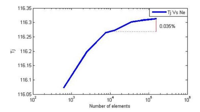
Analysis of mesh independence and verification of the developed numerical model.
Table 2 Junction temperature TJ at different numbers of elements (NE).
| NE | 630 | 2514 | 7518 | 12999 | 36154 | 64825 | 160332 |
|---|---|---|---|---|---|---|---|
| TJ (°C) | 116.1 | 116.2 | 116.26 | 116.27 | 116.3 | 116.31 | 116.31 |
Table 3 The junction temperature of the LED model.
| TJ of our ANSYS model (°C) | TJ of the reference model (°C) | Relative deviation (%) |
|---|---|---|
| 116.270 | 115.780 | 0.421 |
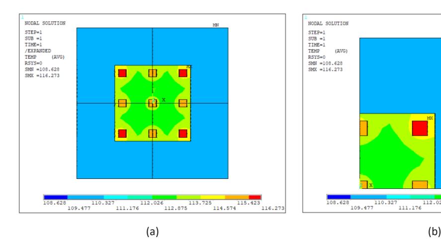
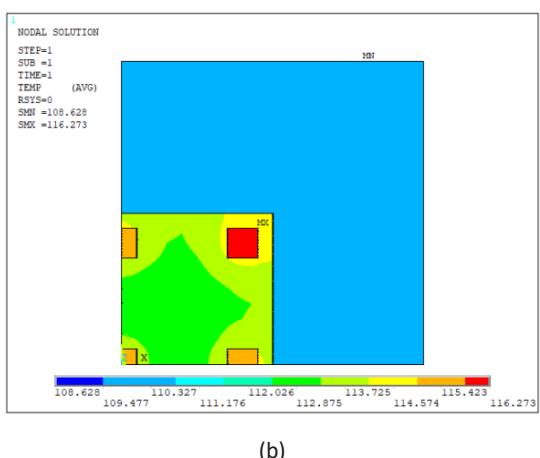
Result of the simulation of a multi- chip LED package: (a) top view and (b) one-fourth of the top view.
Effect of Phosphor Layers on the Thermal Behavior of a COB-LED Module
A phosphor layer will produce additional thermal losses due to the heat generated during the light conversion process. This conversion will certainly lead to an increase in the junction temperature. However, the magnitude of this increase depends on many factors and can vary considerably depending on the specific design of the LED, the materials used, the thermal management and other operating conditions. In order to study the effect of phosphor layers on the thermal behavior, a thermal model of the LED package was studied by adding a homogeneous phosphor layer. We assumed a conformal coating for the LED chip with two identical layers of phosphor (see Figure 6 (a-b)). A quarter of the original LED packaging was used as the simulation area in order to simplify the thermal model. Table 4 shows the list of the constant parameters that were used in our simulation. One phosphor layer in the module had a height of 60 µm and a concentration of 70%. According to reference [4], from which the basic design was derived, the LED chip matrix consumes 3.5 W of electrical energy with a 15% efficiency (0.5 W converted into blue light and 3W converted into heat). Our simulation demonstrated that the junction temperature was approximately 129.17 °C after adding the phosphor layers (see Figure 7), with a significant increase of 11.1%.
Table 4 Material parameters of one phosphor layer.
| Thickness | Concentration | Thermal conductivity | Light conversion | |
|---|---|---|---|---|
| (µm) | (%) | (W/m.K) | efficiency | |
| One Phosphor layer | 60 | 70% | 0.23 | 70% |
Mesh of the ¼ studied model: (a) without phosphor layers and (b) with phosphor layers.
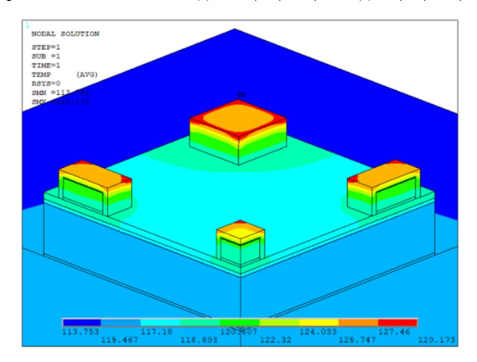
Overall temperature distributions in the multi-chip LED package thermal model with phosphor layers.
Sensitivity Analysis Results
This section discusses the sensitivity results of the LED package based on the Sobol method by investigating the properties of random variables and the laws of probability of the layer materials. According to Table 5, each layer has a Gaussian law of probability to clarify the sensitivity results of the model. The Sobol sensitivity analysis was performed to confirm the interactions between the parameters and quantitatively evaluate the impacts of nine random variable parameters linked to the thermal conductivity of the various material layers of the package. During a genuine industrial project of design and production of a level-2 electronic system based on LED chips, the variations in design parameters (from a thermal perspective) can depend on several factors, including the complexity of the system, the materials used, and thermal performance requirements. These variations include:
- 1. Material thermal properties provided by material manufacturers based on laboratory tests and production specifications.
- 2. Demands related to geometry and dimensions dependent on the fabrication capabilities of the technologies used to produce LED systems.
- 3. The energy dissipated by LEDs and environmental conditions, obtained from laboratory tests.
Our finite element model, which we were able to validate and calibrate, is based on a design concept derived from reference [4], whose design parameters were assumed to be deterministic by the authors. Knowing that the standard deviations of the design parameters of level-2 electronic systems from a thermal perspective can vary between 0.1% and 20%, and lacking the standard deviations of the design parameters from the base design taken from reference [4], we decided to adopt a percentage of 5% for the standard deviations of the 28 design parameters in our model. According to Figure 8, the heat sink, copper, die, and dielectric are the most important factors influencing junction temperature. The rest of the parameters were determined to be insignificant.
| Material components | Laws of Probability | Mean | Standard deviation | |
|---|---|---|---|---|
| LED chip | Gaussian | 130.0 | 130.0 × 5% | |
| Die | Gaussian | 124.0 | 124.0 × 5% | |
| Metallization | Gaussian | 27.0 | 27.0 × 5% | |
| Dielectric | Gaussian | 1.10 | 1.10 × 5% | |
| Die-attach | Gaussian | 57.0 | 57.0 × 5% | |
| Copper | Gaussian | 382.0 | 382.0 × 5% | |
| TIM | Gaussian | 3.0 | 3.0 × 5% | |
| Base | Gaussian | 150.0 | 150.0 × 5% | |
| Heat sink | Gaussian | 150.0 | 150.0 × 5% | |
Table 5 Random variable parameters relative to the of the materials (W/m.K).
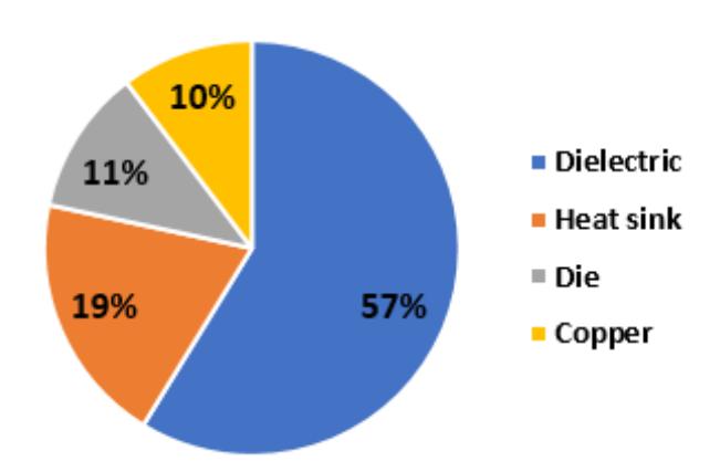
The most affecting parameters on the thermal behavior of the LED package.
Reliability Results
Using the reliability techniques described in the previous section, we used two approximations to solve the integral of the probability of failure Eq. (7), such as MC and FORM/ SORM methodologies. Based on Eq. (8), the performance function is written as G(X, d), where R corresponds to the resistance and S for the load effect. We
reformulated the expression of the performance function according to our study by replacing the resistance by the maximum junction temperature, TJMAX = 120°C and the load effect S by the calculated junction temperature TJ. The performance function G is expressed as:
\[G = T_{\mathsf{JMAX}} - T_{J} \tag{22}\]
Based on the results of the sensitivity study, it was found that the heat sink, copper, die, and dielectric are the most important factors influencing the junction temperature. Because of their impact on the package's thermal behavior, the ambient temperature and the thermal convection coefficient should be treated as random variables. Table 6 lists the random input variables and the distribution parameters that were taken into consideration. Table 7 defines the reliability analysis results using SORM/ FORM an MC methodologies. Due to the SORM method's greater accuracy, the probability of failure obtained from the SORM/FORM approaches was about 20.73%. We performed the study using Monte Carlo sampling to confirm the computed result from the methods used in our research and found that the probability of failure was 20.35% with an error of 0.35%. For reliability computations, this error is acceptable. The standard Monte Carlo sampling method requires 4,000 samples for the simulation and gradually produces the probability of failure over an extremely long time. Instead, the FORM/SORM reliability study only takes a short period for calculation. The standard deviations of 5% on the design parameters and a maximum junction temperature not exceeding TJMAX = 120 ° C generated a probability of failure of 20.73%, which is indeed alarming. However, this result is logical for this test case. Furthermore, it was validated after comparing the FORM/SORM results with those from the Monte Carlo simulation, a classic reference method.
Components Laws of Probability Mean Standard deviation Thermal conductivity (W/m.K) Dielectric Gaussian 1.10 1.1 × 5% Copper Gaussian 382.00 382 × 5% Heat sink Gaussian 150.00 150 × 5% Die Gaussian 124.00 124 × 5% Tamb (°C) Gaussian 25.00 25 × 5% h (W/m2 .K) Gaussian 10.00 10 × 5%
Table 6 Distribution parameters for random variables.
| Variables | Point of conception (FORM) | Point of conception (SORM) | Monte Carlo sampling (4000) | |
|---|---|---|---|---|
| Dielectric | 1.100 | 1.100 | ||
| Thermal conductivity | Heat sink | 150.000 | 150.000 | |
| (W/m.K) | Copper | 385.000 | 385.000 | |
| Die | 124.000 | 127.00 | ||
| Tamb (°C) | 25.270 | 25.270 | ||
| h (W/m2 .K) | 9.610 | 9.60 | ||
| (%) | 82 | 82 | ||
| Pf (%) | 20.73 | 20.73 | 20.35 | |
RBDO
Results of Sensitivity Analysis of the Model Based on Geometric Properties
It is important to identify the design factors that have a significant impact on the junction temperature of the package before going on to the RBDO results. For this reason, a sensitivity study that focused on the geometric parameters was performed. The laws of probability and the parameters of the variables concerning the different thicknesses of the material layers and the distance between the different LED chips (pitch) are listed in Table 8. Figure 9 shows the geometric parameters with the greatest impact on the TJ of the LED package obtained by the Sobol method. Based on this analysis, the following two geometrical parameters (Thickness of heat sink fin and Pitch) were found to have an important effect, and the additional variables are deterministic and have no impact.
Table 8 Law of probability and design variable parameters.
| Parameters | Mean (m) | Laws of Probability | Maximum (m) | Minimum (m) |
|---|---|---|---|---|
| Pitch | 3×10⁻³ | uniform | 3.3×10⁻³ | 0.5×10⁻³ |
| Side substrate | 10×10-3 | uniform | 10×10-3+10×10-3×2.5% | 10×10-3-10×10-3×2.5% |
| Thickness of LED chip | 4×10⁻⁶ | uniform | 4×10⁻⁶+4×10-6×2.5% | 4×10⁻⁶-4×10-6×2.5% |
| Thickness of the metallization | 10×10-6 | uniform | 10×10-6+10×10-6×2.5% | 10×10-6-10×10-6×2.5% |
| Thickness of die | 375×10-6 | uniform | 375×10-6+375×10-6×2.5% | 375×10-6-375×10-6×2.5% |
| Thickness of die-attach | 50×10-6 | uniform | 50×10-6+50×10-6×2.5% | 50×10-6-50×10-6×2,5% |
| Thickness of copper | 127×10-6 | uniform | 127×10-6+127×10-6×2.5% | 127×10-6-127×10-6×2.5% |
| Thickness of dielectric | 75×10-6 | uniform | 75×10-6+75×10-6×2.5% | 75×10-6-75×10-6×2.5% |
| Thickness of base (metal core) | 1000×10-6 | uniform | 1000×10-6+1000×10-6×2.5% | 1000×10-6-1000×10-6×2.5% |
| Thickness of TIM | 50×10-6 | uniform | 50×10-6+50×10-6×2.5% | 50×10-6-50×10-6×2.5% |
| Thickness of heat sink base | 2×10⁻³ | uniform | 2×10⁻³+2×10-3×2.5% | 2×10⁻³-2×10-3×2.5% |
| Thickness of heat sink fin | 18×10-3 | uniform | 18×10-3+18×10-3×2.5% | 18×10-3-18×10-3×2.5% |
| Side of heat sink fin | 1.5×10⁻³ | uniform | 1.5×10⁻³+1.5×10-3×2.5% | 1.5×10⁻³-1.5×10-3×2.5% |
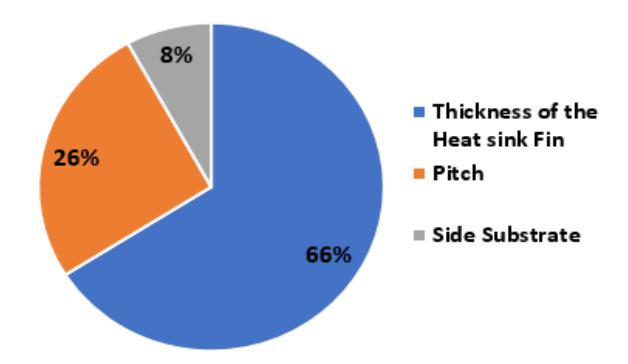
Figure 9 The geometric parameters with the greatest impact on the \(T_1\) of the model.
RBDO Results
In this part of the study, the Sequential Quadratic Programming (SQP) tool in the MATLAB program was used to solve the optimization problem. In our study, six variables were investigated: four random variables symbolized by \(X_r\) and two design parameters \(X_d\), i.e., the pitch and the thickness of the heat sink fin based on the results of the sensitivity analysis. Table 8 defines the mean, minimum, and maximum values required to solve this issue. The optimization problem consisted of finding the vector design \(X_d\) that minimizes the probability of failure of the system under the cost constraint corresponding to the thermal resistance. The RBDO results for the formulation in Eq. (20) are summarized in Table 9. This table illustrates the initial and optimal points of the variables. The reliability level was 91% compared to 80% of the original design, while minimizing the probability of failure, the junction temperature, and the thermal resistance of the model. Additionally, Figure 10 illustrates the package's thermal behavior to show the advantages of the optimal design chosen and established by this study. Since the difference is so minimal, it is assumed that the junction temperature of several chips arranged on the same substrate should be constant.
Table 9 RBDO results.
| Variables | Initial design | Optimal design |
|---|---|---|
| Pitch (m) | \(3 \times 10^{-3}\) | \(2.384 \times 10^{-3}\) |
| Thickness of heat sink fin (m) | \(18 \times 10^{-3}\) | \(18.4 \times 10^{-3}\) |
| TJ (°C) | 116.270 | 114.110 |
| Rth (°C/W) | 91.270 | 89.00 |
| Pf (%) | 20 | ≈9 |
| Reliability Level (%) | 80 | ≈91 |
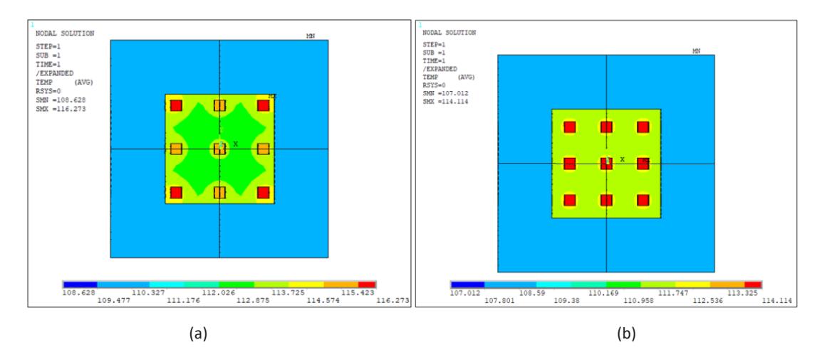
Simulation results of the initial (a) and optimal (b) design of the multi-led chip package.
Conclusion
In this paper, we examined the thermal behavior of an LED package using a validated 3D finite-element model. The structure of the model included a heat sink, substrate, thermal grease, and LED chip. The following is a summary of our main conclusions.
A sensitivity analysis approach was proposed to assess the variables influencing the thermal behavior of the LED package. The Sobol sensitivity analysis method was used in this study, which made it possible to identify the most sensitive factors towards thermal behavior. These factors are: the thermal conductivity of copper, the heat sink, and the dielectric. The junction temperature of the model was not affected by the other components. Then, to identify a reliable and optimal design, an optimization-reliability analysis was carried out using the MATLAB optimization toolbox and the ANSYS finite-element software to obtain the results. The reliability level was evaluated using two approximation methods: FORM and SORM. After that we performed the reliability study using Monte Carlo sampling to confirm the computed outcome from the FORM and SORM methods.
A probabilistic model was developed utilizing the MATLAB software RBDO to minimize the objective function subject to various constraints and to simultaneously evaluate the reliability level. It was able to establish new design parameters for the LED package by using the RBDO technique. The results obtained showed that the RBDO approach is effective in suggesting a design that conforms with reliability and performance requirements. By using this optimization, we were able to increase reliability from 80% to 91%, lower junction temperature, lower thermal resistance, and reduce the failure probability of the original design from 20% to 9%.
Compliance with ethics guidelines
The authors declare that they have no conflict of interest or financial conflicts to disclose.
This article does not contain any studies with human or animal subjects performed by the any of the authors.
Nomenclature
C = heat capacity (J/kg.K) d = design variables
f0 = average value of the model output fi(Xi) = output caused by Xi as a parameter
fij(Xi,Xj) = output produced by the interaction of Xi and Xj
G(X,d) = performance function
h = thermal convection coefficient (W/m2 .K)
mR = mean of the effect of resistance mS = mean of the effect of load Pf = probability of failure Rth = thermal resistance (°C/W)
V(Y) = total variance of the model output
X = random variables
Xd = vector of design variables
Y = output of model (d) = index of reliability
= thermal conductivity (W/m.K)
= density (kg/m3 )
R = standard deviation of the effect of resistance S = standard deviation of the effect of load
() = standard Gaussian cumulative distribution function
Subscripts
amb = ambient d = design J = junction
Jmax = junction maximum
r = random th = thermal