
Introduction
The islands of Bangka and Belitung in Indonesia are part of the Southeast Asian tin belt composed by the intrusion of a granite pluton that is rich in tin mineralization [1, 2]. In granite rock that carries tin mineralization, particularly in alluvial deposits, silica is abundantly present as gangue mineral, which can be mined and beneficiated.
During the on-land alluvial tin mining activities carried out on the islands of Bangka and Belitung, the mineral processing only uses water with a separation method that relies on the specific gravity of the material. This means material that does not contain tin or other heavy minerals will be returned to its original location, so that there are no significant topographical changes. This shows that no chemical process are involved and few changes in mineral characteristics occur when mining tin [3]. Based on the Indonesian government's regulations, the pile of this material is not included in the category of mine tailings material but is rather called a residual of mineral processing or mineral washing. Thus, it is permissible and feasible to mine and process this material again [4, 5].
Residual materials from mineral processing in tin mining generally have several types of mineral content, which can produce valuable materials when further processed. One such valuable material, which is present in large amounts, is quartz sand or silica (SiO2). The products from quartz sand are miscellaneous and beneficial, and can be applied in things
such as glass, water filter makers, ceramic tile-making materials, metal or metal tile-making materials, which is generally beneficial for the manufacturing industry [6]. Thus, considering the potential and usefulness of quartz sand, it is valuable to evaluate and estimate the resources of quartz sand from the residual of alluvial tin processing.
Geostatistics is a scientific discipline introduced by Matheron in 1971, who studied the theory and application of regionalized variables in various natural phenomena. A variable is said to be regionalized when it is distributed spatially and characterizes a certain phenomenon, such as mineral content in a mineralized zone. Estimating the content and amount of residual materials from mineral processing is generally difficult due to their high variability, which results in a high degree of uncertainty in resource estimation.
Alluvial deposits in Indonesia have been studied using three geostatistical approaches to model the resource uncertainty [7, 8]. One of these approaches, namely global estimation variance (GEV), was used in the present study. GEV is a concept that characterizes the error associated with a particular sampling pattern and the geometry to be estimated [9]. Some researchers have used GEV for evaluating coal resources. In GEV, an extension variance is used to calculate the relative error when estimating a block using only one sample located in the middle of the block [10-12]. In this study, the error rate obtained from GEV was incorporated with the kriging variance (KV), which was obtained from the estimation using the ordinary kriging (OK) method. KV is a measure of the uncertainty of the estimation results, where the value indicates the level of confidence in the estimation results. The incorporation of two geostatistical approaches is interesting to optimize the drill hole spacing. After that, resource estimation from such drill hole spacing are expected to represent the measured and indicated categories, so they can be converted to the reserves.
Materials and Methods
The study sites were in land alluvial tin mining areas located on Bangka Island, named Block I, and on Belitung Island, named Block II, as shown in Figure 1.
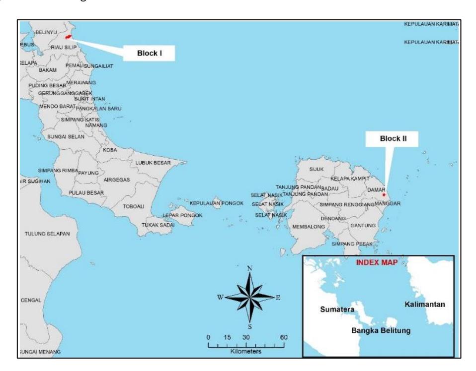
Location map of study sites.
The data collected were in the form of drilling samples with an average depth of 7 to 8 m. The base map of drill hole data is depicted in Figure 2(a) for Block I and Figure 2(b) for Block II. The drilling results are summarized in Table 1.
The methods used in this study involved statistical analysis to see the parameters of data distribution, i.e., mean, median, mode, skewness, and variance. Variogram analysis was used to determine the spatial structure parameters, i.e., nugget variance, sill variance, and range. The GEV was calculated to see the global relative error based on certain drill hole spacing scenarios. Then a block model was created to produce the kriging variances and to obtain the measure of uncertainty, which indicates the level of confidence in the estimation results for resource categorization.
Data
Drilling data was taken to obtain a reference sample, i.e., collar data, assays, lithology, and surveys from residual processing materials. In Block I of Bangka, there were a total of 127 drill holes with an average depth of 8.01 m and a total depth of 1,016.65 m, while in Block II of Belitung, there were a total of 68 drill holes with an average depth of 7.74 m and a total depth of 526.35.
Table 1 Summary of drill holes.
| Site | Number of drill holes | Average depth (m) | Depth range (m) Min. Max. | Total depth (m) | |
|---|---|---|---|---|---|
| Block I | 127 | 8.01 | 0.85 | 15.80 | 1,016.65 |
| Block II | 68 | 7.74 | 5.10 | 9.30 | 526.35 |
Base map of the distribution of drill holes (marked as green dots) overlaid onto aerial photography at: (a) Block I and (b) Block II.
Univariate Statistics and Variograms
Univariate statistical analysis was performed by looking at the mean, median, standard deviation, skewness, and variance. This shows what the data pattern and distribution are like. A variogram was used to see the spatial autocorrelation of the data and as the input parameter to calculate GEV and KV. In this study, GEV was only performed for the thickness and the grade accumulation variables, where the grade accumulation is the product of thickness multiplied by grade.
A variogram was used to see the spatial variability and correlation between two data separated by a certain distance. Mathematically, the experimental variogram, y(h), is expressed in Eq. (1) as follows [13, 14]:
\[\gamma(h) = \sum_{i=1}^{n} [Z(X_i) - Z(X_i + h)] 2 / 2N(h)\] (1)
where \(Z(x_i)\) is a data value at location \(x_i\), and \(Z(x_i + h)\) is a data value at location \(x_i\) separated by distance h.
Construction of the experimental variogram was performed using the public domain software SGeMS (Stanford Geostatistical Earth Modeling Software) by applying an omnidirectional variogram. Then a fitting model was constructed to determine the geostatistical parameters nugget variance (Co), sill variance (C1), and range or area of influence (a). The total nugget variance and sill variance was set close to the population variance. The choice of omnidirectional variogram refers to the distribution of quartz sands in residual processing material, which tends not to have a certain anisotropy.
Variography analysis shows that the SiO<sub>2</sub> grade had a high-to-extreme nugget ratio. Consequently, the SiO<sub>2</sub> grade was not directly used for the GEV calculation and interpolation. The thickness and grade accumulation were considered sufficient to represent the data for resource estimation using geostatistics. The statistical analysis of thickness and grade accumulation is summarized in Table 2, while a summary of the variogram model parameters is shown in Table 3.
| Block I | Block II | |||||
|---|---|---|---|---|---|---|
| Parameters | Thickness Grade accumulation | Thickness | Grade accumulation | |||
| (m) | (%.m) | (m) | (%.m) | |||
| Mean | 8.00 | 794.64 | 7.61 | 750.19 | ||
| Median | 7.90 | 789.84 | 7.75 | 754.42 | ||
| Standard deviation | 2.63 | 261.74 | 0.96 | 95.98 | ||
| Sample variance | 6.90 | 68,506 | 0.93 | 9,211 | ||
| Skewness | -0.10 | -0.09 | -0.32 | -0.32 | ||
| Coefficient of variation | 0.33 | 0.39 | 0.13 | 0.13 | ||
| Min. | 0.85 | 84.91 | 5.00 | 492.16 | ||
| Max. | 15.80 | 1.576.40 | 9.10 | 906.13 | ||
Table 2 Statistical summary of thickness and grade accumulation.
Table 3 Summary of variogram model (spherical) parameters.
| Sites | Parameters | SiO₂ grade (%) | Thickness (m) | Grade accumulation (%.m) |
|---|---|---|---|---|
| Nugget variance | 0.65 | 4.20 | 40,000 | |
| Block I | Sill variance | 0.25 | 2.80 | 28,600 |
| Range (m) | 95 | 300 | 250 | |
| Nugget variance | 3.50 | 0.40 | 3,500 | |
| Block II | Sill variance | 1.20 | 0.60 | 5,900 |
| Range (m) | 65 | 320 | 250 |
Global Estimation Variance (GEV)
Global estimation variance (GEV) is used to find the global relative error based on the results of the extension variance at a certain grid size that corresponds to the drill hole spacing. The extension variance is a function of the variogram model based on existing data and the scenario of grid or block size. Practically, the extension or estimation variance is calculated for grids or blocks whose size is the same as the average drill hole spacing. Then the block is discretized to a size of \(5 \times 5\), so that there are 25 regularly spaced nodes in the block. Eq. (2) was used to calculate the estimation variance (\(\sigma^2_E\)):
\[\sigma^{2}_{E} = \bar{\gamma}(S, V) - \bar{\gamma}(V, V) - \gamma(S, S) \tag{2}\] where ̅(, ) is the point-to-block average variogram, ̅(, ) is the block-to-block average variogram, and (, ) is the point-to-point variogram. Meanwhile, GEV was obtained from Eq. (3) as follows:
\[GEV = \frac{\sigma^2 e}{N} \tag{3}\] where 2 e is the estimation variance and is the number of grids or blocks. At the study site, various grid sizes of 50 × 50 up to 300 × 300 m were applied. Then, assuming a 95% confidence level, the relative error was calculated by Eq. (4) as follows:
\[Relative\ error\ =\ \frac{\pm 2\sqrt{GEV}}{\bar{z}}\ \times\ 100\% \tag{4}\] where is the average (mean) of the population. The plotting of the relative error was correlated to the drill hole spacing scenario, so the confluence of the two parameters could be a reference for resource categorization followed by drill hole spacing optimization. The following assumption (Eq. (5)) was used for resource categorization based on the relative error:
Measured \[10\% \le \text{Indicated } 20\% \le \text{Inferred}\] (5)
Block Model and Resource Estimation
The block model for resource estimation was built using a prototype model with a grid or cell size of 25 × 25 × 5 m. The prototype model was limited by the size and coordinate point of the boundary of the block to be estimated, where the initial coordinates (x, y, z) of the block boundary, as well as the number of cells in the x, y, z direction were used as the input data in creating the prototype model. The created model filled the entire area that was defined with empty cells that matched the specified size and number of cells. An image of the prototype model is shown in Figure 3(b).
Example of the block model (Block II): (a) quartz sand solid wireframe, (b) quartz sand prototype model (white line) with a grid or cell size of 25 × 25 × 5 m, which is limited by the size/coordinate points of the block boundaries to be estimated.
The prototype model that was created previously, which contained empty cells, filled the solid model of the wireframe (see Figure 3(a)). Subsequently, the maximum number of splits used in filling the wireframe was determined. A split is a division of the cell size that has previously been determined in creating the prototype model. The estimation of quartz sand resources used a split number of 1, which means that the block model applied a sub-cell size of 12.5 × 12.5 × 5 m, filling the wireframe with the prototype model (see Figure 4).
The resource estimation was performed using the ordinary kriging (OK) method, which is a linear geostatistical interpolator method that is commonly used to estimate unknown values at locations (grids or cells) using neighbourhood samples. This method involves calculating the weighted average of adjacent samples as data points by considering the spatial distances and correlations [15-17].
Interpolation of the block model was not carried out directly on SiO2 grades, because their variogram structure had a high-to-extreme nugget ratio, as previously mentioned, while the variogram structures of thickness and grade accumulation was more stationary with a relatively low nugget ratio. This is why the estimation of SiO2 grade was indirectly performed using kriging estimation of the thickness and the SiO2 grade accumulation expressed in Eq. (6) and Eq. (7) as follows:
\[SiO_2\] grade accumulation = Composited \(SiO_2\) grade × Thickness (6)
\[[Composited SiO2 grade]^* = [SiO2 grade accumulation]^K / [Thickness]^K\] (7)
where [Composited SiO2 grade]* is the estimated SiO2 grade, [SiO2 grade accumulation]K is the kriged estimate of the grade accumulation, and [Thickness]Kis the kriged estimate of the thickness.
Example of quartz sand sub-cell processing (Block II).
The general formula of linear estimation is written in Eq. (8) as follows:
\[Z(V)^* = \sum \lambda_i \times Z(x_i)\] (8)
where Z(V)* is the estimated value in the grid or cell V, Z(xi) is the data value used for interpolation at location xi, and λi is the kriging weight, which is a function of the variogram parameters. Meanwhile, to calculate the weight λi, the ordinary kriging (OK) system is expressed in Eq. (9) as follows:
\[\sum \lambda_{i} \times \gamma(x_{i}, x_{i}) + \mu = \overline{\gamma}(x_{i}, V) \tag{9}\] where \(\gamma(x_i, x_j)\) is the variogram between data values at locations \(x_i\) and \(x_j\), \(\mu\) is the Lagrange number, \(\overline{\gamma}(x_i, V)\) is the average variogram of data at point \(x_i\) to grid or cell V. The uncertainty of the kriged estimate is represented by a kriging variance or estimation variance (\(\sigma_K\)) in Eq. (10) as follows:
\[\sigma_{K} = -\overline{\gamma}(V, V) + \mu + \Sigma \lambda_{i} \times \overline{\gamma}(x_{i}, V)\] (10)
where \(\overline{\gamma}(V, V)\) is the average variogram within cell V, \(\mu\) is the Lagrange number, \(\overline{\gamma}(x_i, V)\) is the average variogram of the data at point \(x_i\) to cell V.
Resources Categorization
The resource categorization was carried out using the estimation variance or error variance based on the kriging variance from the results of estimated thickness and grade accumulation. In this process, the interpolation results were also cropped for the area of interest (AoI) by removing holes or underbellies in all blocks, as depicted in Figure 6(a). Because the interpolation of SiO<sub>2</sub> grade was not performed directly using the OK method, their estimation variance was calculated based on Eq. (11) as follows [18, 19]:
\[\frac{\sigma^2 m_x m_y}{(m_x m_y)^2} = \frac{\sigma^2 m_x}{m_x^2} + \frac{\sigma^2 m_y}{m_y^2} + 2\rho_{m_x m_y} \frac{\sigma_{m_x}}{m_x} \frac{\sigma_{m_y}}{m_y}\](11)
where \(m_x m_y\) is the kriging estimate of the grade accumulation, \(\sigma^2 m_x m_y\) is the kriging variance of the grade accumulation, \(m_x\) is the kriging estimate of the thickness, \(m_y\) is the kriging estimate of the SiO<sub>2</sub> grade, \(\sigma^2 m_x\) is the kriging variance of the thickness, \(\sigma^2 m_x\) is the kriging variance of the SiO<sub>2</sub> grade, and \(\rho_{m_x m_y}\) is the correlation coefficient between thickness and grade. As the kriging variance of the SiO<sub>2</sub> grade could be obtained directly from the kriging estimation, the estimation variance of the SiO<sub>2</sub> grade (\(\sigma^2 grade\)) was obtained from Eq. (11), which was modified into Eq. (12) as follows:
\[\sigma^{2} grade = \left[ \frac{\sigma^{2} grade \ accumulation}{(est.grade \ accumulation)^{2}} - \frac{\sigma^{2} thickness}{(est.thickness)^{2}} \right] \times (est. \ grade)^{2}\] (12)
where \(\sigma^2\) grade is the estimation variance of the SiO<sub>2</sub> grade, \(\sigma^2\) grade is the kriging variance of the grade accumulation, \(\sigma^2\) thickness is the kriging variance of the thickness, est. grade accumulation is the kriged estimate of the grade accumulation, est. thickness is the kriged estimate of the thickness, and est. grade is the estimate of the SiO<sub>2</sub> grade from Eq. (7).
The estimation variance of the SiO<sub>2</sub> grade was then converted to a relative standard deviation of error, known as the relative kriging standard deviation (RKSD) (Eq. (13)) as follows:
\[RKSD = \pm 2 \times \frac{\sigma_{grade}}{est.grade} \times 100\%\] (13)
where the multiplier factor of 2 is the coefficient for confidence level 95% assuming that the error distribution is normal. RKSD is a parameter used in geostatistical estimation to assess the uncertainty or variability of predictions made by the kriging interpolation method. RKSD provides a measure of the reliability of estimates by calculating the standard deviation of the difference between the estimated value and the true value at each location relative to the estimated results in each grid or cell. A relatively high RKSD indicates relatively large uncertainty. In other words, it produces a relatively lower confidence of the kriging estimation results, while a relatively low RKSD indicates a relatively high level of confidence in the estimation results. The RKSD is then incorporated in the GEV in order to produce the optimum drill hole spacing for resource categorization.
Results and Discussion
The first resource evaluation was carried out based on the results of the drill hole spacing analysis (DHSA), using the relative error rates from GEV on the variables of thickness and grade accumulation to produce the optimum drill hole spacing. Plotting the relative error (%) with the assumption that the maximum relative error was 10% and 20% for the measured and indicated resources category, respectively. Determination of the optimum drill hole spacing for Block I and Block II can be seen in Tables 4 and 5, respectively. The plotting results of the relative error as a function of drill hole spacing are shown in Figure 5.
Table 4 Summary of GEV calculation in Block I.
| Parameters | Drill hole spacing (m) | N | 𝛾̅(S, V) | 𝛾̅(V, V) | (S, S) | 2 E | GEV | Relative error (%) |
|---|---|---|---|---|---|---|---|---|
| 50 | 101 | 4.47 | 4.39 | 0.00 | 4.54 | 0.04 | 5.30 | |
| 100 | 58 | 4.71 | 4.90 | 0.00 | 4.52 | 0.08 | 6.98 | |
| 150 | 37 | 4.97 | 5.23 | 0.00 | 4.72 | 0.13 | 8.93 | |
| Thickness (m) | 200 | 33 | 5.22 | 5.53 | 0.00 | 4.91 | 0.15 | 9.65 |
| 250 | 26 | 5.45 | 5.80 | 0.00 | 5.11 | 0.20 | 11.09 | |
| 300 | 21 | 5.67 | 6.02 | 0.00 | 5.32 | 0.25 | 12.59 | |
| 50 | 101 | 43,316 | 42,855 | 0.00 | 43,776 | 433 | 5.24 | |
| 100 | 58 | 46,305 | 48,618 | 0.00 | 43,991 | 758 | 6.93 | |
| Grade | 150 | 37 | 49,533 | 52,526 | 0.00 | 46,540 | 1,257 | 8.93 |
| Accumulation (%.m) | 200 | 33 | 52,469 | 55,955 | 0.00 | 48,984 | 1,484 | 9.70 |
| 250 | 26 | 55,199 | 58,751 | 0.00 | 51,646 | 1,986 | 11.22 | |
| 300 | 21 | 57,669 | 60,846 | 0.00 | 54,492 | 2,594 | 12.82 |
Table 5 Summary of GEV calculation in Block II.
| Parameters | Drill hole spacing (m) | N | 𝛾̅(S, V) | 𝛾̅(V, V) | (S, S) | 2 E | GEV | Relative error (%) |
|---|---|---|---|---|---|---|---|---|
| 50 | 61 | 0.56 | 0.46 | 0.00 | 0.66 | 0.01 | 2.74 | |
| 100 | 41 | 0.50 | 0.54 | 0.00 | 0.46 | 0.01 | 2.80 | |
| 150 | 21 | 0.56 | 0.61 | 0.00 | 0.50 | 0.02 | 4.07 | |
| Thickness (m) | 200 | 16 | 0.61 | 0.67 | 0.00 | 0.54 | 0.03 | 4.84 |
| 250 | 10 | 0.65 | 0.73 | 0.00 | 0.58 | 0.06 | 6.34 | |
| 300 | 8 | 0.70 | 0.77 | 0.00 | 0.62 | 0.08 | 7.34 | |
| 50 | 61 | 4,175 | 4,260 | 0.00 | 4,090 | 67. | 2.18 | |
| 100 | 41 | 4,785 | 5,257 | 0.00 | 4,313 | 105 | 2.73 | |
| Grade | 150 | 21 | 5,444 | 6,056 | 0.00 | 4,831 | 230 | 4.04 |
| accumulation (%.m) | 200 | 16 | 6,044 | 6,760 | 0.00 | 5,328 | 333 | 4.87 |
| 250 | 10 | 6,603 | 7,337 | 0.00 | 5,868 | 586 | 6.46 | |
| 300 | 8 | 7,110 | 7,774 | 0.00 | 6,446 | 805 | 7.57 |
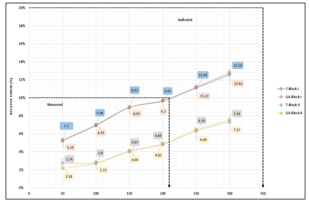
Plotting the relative error from GEV as a function of the drill hole spacing scenario in Block I and Block II. Note: T = thickness; GA = grade accumulation
Based on the plotting of the relative error, as the relative error in Block I was larger than in Block II, it was considered to represent the optimum drill hole spacing for both sites. Therefore, the optimum drill hole spacing for the measured and indicated resources based on grade accumulation was determined to be 210 m and 325 m, respectively. The optimum drill hole spacing considering the SiO2 grade was then estimated using the ratio of variogram range between SiO2 grade and grade accumulation as summarized in Table 6. As the average ratio of their variogram range was about 0.32 for both blocks, the optimum drill hole spacing for SiO2 grades was estimated to be about 32% of the optimum drill hole spacing of grade accumulation, i.e., 65 m and 100 m for the measured and indicated resources, respectively.
Table 6 Summary of variogram range (in meters) ratio between SiO2 grade and grade accumulation.
| Sites | SiO2 grade (%) | Grade accumulation (%.m) | Ratio |
|---|---|---|---|
| Block I | 95 | 250 | 0.38 |
| Block II | 65 | 250 | 0.26 |
| Average | 80 | 250 | 0.32 |
The resource categorization based on RKSD is shown in Figures 6(b) and 7(b), where the categorization is deducted from the statistical distribution of RKSD, i.e., measured if RKSD 5%, indicated if 5%< RKSD 10%, and inferred if RKSD >10%. When we applied the RKSD distribution for resource categorization, as shown in Figures 6a and 7a, we could identify the range of existing drill hole spacings associated with each resource category at both sites, as summarized in Table 7. The incorporation of the RKSD distribution and the existing drill hole spacings for both sites showed that Block I exhibited almost 50% shorter drill hole spacings per resource category compared to Block II.
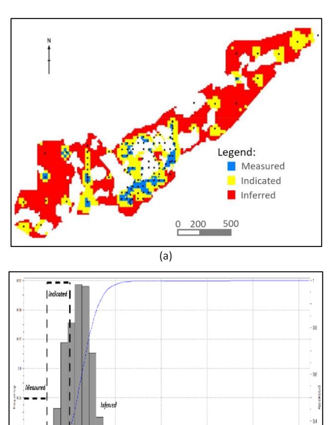
Resource categorization for Block I: (a) resource categorization map based on RKSD, (b) statistical distribution of RKSD with three resource categories.
(b)
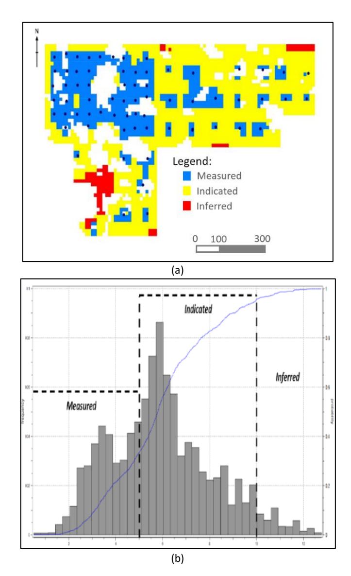
Resource categorization for Block II: (a) resource categorization map based on RKSD, (b) statistical distribution of RKSD with three resource categories.
Table 7 Incorporation of RKSD into the range of drill hole spacings for each resource category.
| Sites | Resource categories | ||
|---|---|---|---|
| RKSD ≤5% (measured) | 5% RKSD ≤10% (indicated) | RKSD >10% (inferred) | |
| Block I | 25–35 m | 35–65 m | >65 m |
| Block II | 50–75 m | 75–100 m | >100 m |
All estimation maps of thickness are shown in Figure 8(a) for Block I and in Figure 9(a) for Block II, grade accumulation is shown in Figure 8(b) for Block I and in Figure 9(b) for Block II, and the SiO2 grades are shown in Figure 8(c) for Block I and in Figure 9(c) for Block II. These maps were deducted based on the area of interest in the form of cropping the areacovering waterbody and also limiting the outermost estimation area by half of the distance of the outer existing drill hole spacing.
The estimation of quartz sand resources and their categorization based on the RKSD distribution for both sites is summarized in Table 8. A total of 13.41 Mt quartz sand with an average grade of SiO2 99.17 is reported in Block I, and a total of 5.73 Mt quartz sand with an average grade of SiO2 98.73% is reported in Block II. Excluding the inferred resource category, the quartz sand resources will probably be converted to the reserves after performing a mine planning and mineral processing study.
Based on the RKSD comparison of the two sites, the variations in drill hole spacing for each resource category were quite different. Factors that may have caused this difference are mining intensity or the geological conditions at the two sites on two different islands. Different mining intensities depending on the company's plans or production targets cause differences in layer thickness as well as the number of waterhole areas. The greater number of waterhole areas in Block I caused the drill hole or sampling pattern to be more irregular or spatially less continuous. The implication for the estimation results is that the area of measured resources in Block I has less coverage than the area in Block II. From a statistical point of view, the thickness and grade accumulation in Block I are more dispersed compared to those in Block II.
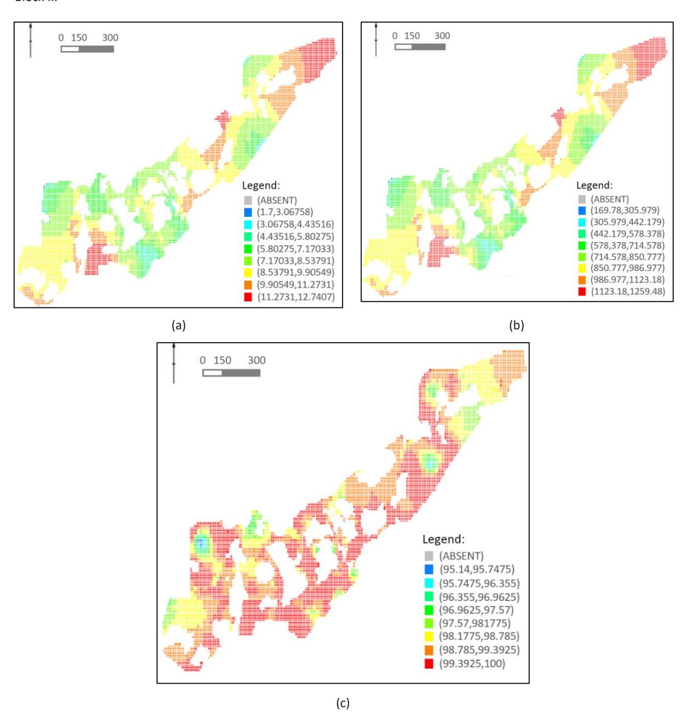
Resource estimation maps for Block I: (a) estimated thickness, (b) estimated grade accumulation, (c) estimated SiO2 grade.
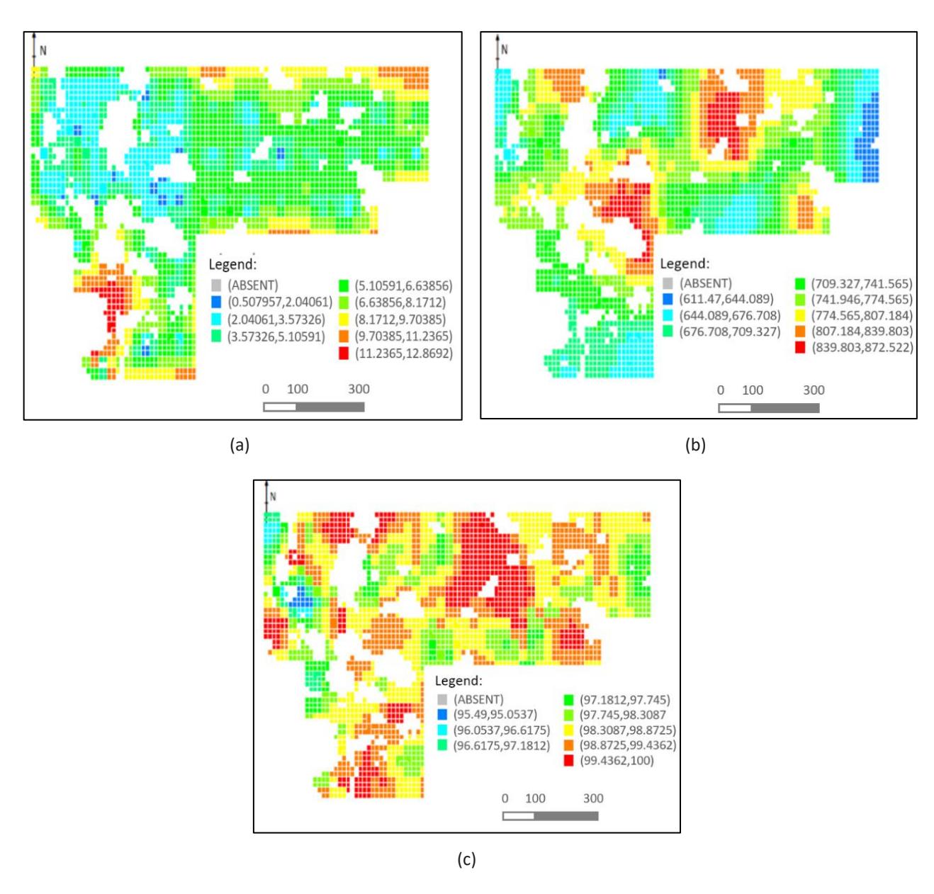
Resource estimation maps for Block II: (a) estimated thickness, (b) estimated grade accumulation, (c) estimated SiO2 grade.
Table 8 Summary of quartz sand resources for both study sites.
| Sites | Categories | Volume (× 106 m3 ) | Dry density (t/m3 ) | Tonnage (Mt) | Average grade (%) |
|---|---|---|---|---|---|
| Measured | 0.58 | 1.53 | 0.88 | 99.76 | |
| Indicated | 2.43 | 1.53 | 3.72 | 99.31 | |
| Block I | Inferred | 5.76 | 1.53 | 8.81 | 99.06 |
| Total | 8.77 | - | 13.41 | 99.17 | |
| Measured | 1.26 | 1.54 | 1.94 | 98.75 | |
| Indicated | 2.28 | 1.54 | 3.51 | 98.73 | |
| Block II | Inferred | 0.18 | 1.54 | 0.28 | 98.62 |
| Total | 3.72 | - | 5.73 | 98.73 |
In terms of geological conditions, Block I is located in an area where rock types such as granite and granodiorite are generally found, so that the silica sand at this location tends to have a high percentage of silica (SiO2) (see Figure 8(c)). This high percentage of silica is due to the immediate weathering of granite and granodiorite. Meanwhile, Block II has a relatively lower percentage of silica (see Figure 9(c)) because it is located in an area where sandstone, silt, shale, and the majority of sedimentary rock are found as bedrock. Hence, the silica in Block II is predominantly sedimentary rock silica that has been undergoing a process of re-release. Statistically, a higher percentage of silica will generate higher variability or less spatial continuity.
Conclusion
Based on this study on resource evaluation of quartz sand as residual material from on-land alluvial tin processing using geostatistical approaches, the following conclusions can be drawn. The resource estimation using geostatistics of the SiO2 grade could not be performed directly because its spatial distribution showed a high nugget ratio. Thus, the grade accumulation as the product of composited SiO2 grade multiplied by layer thickness was used for estimation. Drill hole spacing analysis (DHSA) based on the global estimation variance (GEV) showed that the optimum drill hole spacing for grade accumulation at Block I was chosen to represent the general optimum spacing at both sites because they showed a shorter spacing. The relative kriging standard deviation (RKSD), which was deducted from the estimation variance of the SiO2 grade, coincided with the drill hole spacing for each resource category, where Block I showed almost half shorter spacing compared to Block II. The result of the quartz sand resource estimation for both sites showed that the material tonnage at Block I was more than twice that of Block II, while the SiO2 grade was also higher. The total estimated resources of quartz sand amounted to 13.41 Mt with an average SiO2 grade of 99.17% in Block I and 5.73 Mt, with an average SiO2 grade of 98.73% in Block II. These provide high prospects for further mining and beneficiation. Overall, the geostatistical methods used in this study were effective in evaluating the existing drill hole spacing of quartz sand from the residual material of mineral processing as well as to estimate the resources along with their categories and uncertainty.
Acknowledgement
Sincere thanks to the Faculty of Mining and Petroleum Engineering, Bandung Institute of Technology for the financial support through the PPMI 2023 research program. Thanks, are also extended to PT Timah Tbk. for their excellent support and facilitating this study.
Compliance with ethics guidelines
The authors declare that they have no conflict of interest or financial conflicts to disclose.
This article does not contain any studies with human or animal subjects performed by any of the authors.