
Introduction
Active control systems can be implemented in structures to reduce the responses from dynamic loads. The control forces in active control systems are determined by a control algorithm. One of the known algorithms that has been used in control systems is the Linear Quadratic Regulator (LQR) algorithm, which minimizes the objective function with corresponding weight matrices for responses and forces. State variables in the form of velocities and displacements are required to calculate the control forces using LQR. However, the number of sensors used in structures is usually limited, so the measurement of full-state variables is rarely feasible. Therefore, a state observer is needed to handle the limited number of sensors, although it also adds computation time and delay in the control system [1].
There have been various developments in using artificial intelligence (AI) based controllers to address the problems that arise from LQR-based controllers. Pei-Ching Chen et al. [12] studied a machine learning-based control using Multi-Layer Perceptron (MLP) and Autoregressive Exogenous (ARX) models for a ten-story building validated with an experiment using a single degree of freedom (SDOF) model. The study demonstrated that both MLP and ARX models were able to learn and emulate LQR optimized with Symbiotic Organism Search (SOS). Bani and Ghaboussi [3] utilized a neural network control algorithm on a nonlinear steel frame model with three degrees of freedom. Moreover, Bani [4] employed a neural network controller to reduce wind-induced vibrations in a tall building using an active mass damper. An Artificial Neural Network (ANN) has also been successfully applied to control a bridge by Cho [5]. Other ANN-based controller studies, conducted by Kim et al. [6], Kim and Lee [7], also Rao and Datta [8], have shown great results.
Another control model was studied by Pourzeynali et al. [9]. Theirstudy used a Genetic algorithm and Fuzzy Logic (GFLC) for an Active Tuned Mass Damper (ATMD) implemented in an eleven-story building. Numerically, it showed that GFLC is effective in reducing the building's response. A fuzzy controller has also been studied by Samali et al. [10] to reduce the crosswind response of a 76-story tall building. Furthermore, optimization and tuning of a fuzzy logic controller with multiple objectives has been studied by Ahlawat and Ramaswamy [11].
Most of the studies focused solely on either a neural network model or fuzzy logic. Furthermore, many of these studies either lacked experimental validation or only conducted an experiment on a single-degree-of-freedom model. This paper investigated the effectiveness of both a fuzzy logic controller and a neural network-based controller for an active mass damper. The study involved implementing a recently developed optimization algorithm, SOS, on a fuzzy logic controller and conducting experiment validation on a three-story building model. The objectives consisted of designing AI-based control models for a structure; analysing the practicality and effectivity of the corresponding control models; and determining the optimal control AI-based control model and validating it with experiments.
Numerical Modeling
Equation of Motion
The equations of motion for an n-degrees-of-freedom (NDOF) shear building equipped with an active mass damper (AMD) on top of the building can be formulated as follows in Eq. (1):
\[\mathbf{M}\ddot{\mathbf{x}} + \mathbf{C}\dot{\mathbf{x}} + \mathbf{K}\mathbf{x} = \mathbf{\gamma}u(t) + \mathbf{\delta}\ddot{x}_g(t) \tag{1}\] where M, C, and K are n x n matrices with respect to the mass, damping, and stiffness of the building, respectively; x(t) is a n x 1 vector that represents the absolute displacements at each floor; u(t) is the control force of AMD; is a n x 1 vector that indicates the location on which the control force of AMD is imposed to the structure; is a n x 1 vector with all elements equal to negative mass of each story; and ̈ is the ground acceleration. If the states are defined as (t) = [(t) ̇(t)] T , then the state-space formulation of the structure can be written as follows in Eq. (2):
\[\dot{\mathbf{Z}}(t) = \mathbf{A}\mathbf{Z}(t) + \mathbf{B}_{\mathbf{u}}u(t) + \mathbf{B}_{\mathbf{r}}\ddot{\mathbf{x}}_{g}(t)\] (2)
where the system matrix A, the control force distribution matrix Bu, and the disturbance location matrix Br are expressed in Eq. (3):
\[\mathbf{A} = \begin{bmatrix} \mathbf{0} & \mathbf{I} \\ -\mathbf{M}^{-1} & -\mathbf{M}^{-1} \mathbf{C} \end{bmatrix}; \quad \mathbf{B}_{\mathbf{u}} = \begin{bmatrix} \mathbf{0} \\ \mathbf{M}^{-1} \boldsymbol{\gamma} \end{bmatrix}; \quad \mathbf{B}_{\mathbf{r}} = \left\{ \begin{matrix} \mathbf{0} \\ \mathbf{M}^{-1} \boldsymbol{\delta} \end{matrix} \right\}\](3)
Structure Description
A three-story prototyped-sized building model was used in this study, as shown in Figure 1.
The three-story building model.
The specimen was a small-scale aluminium alloy structure with three degrees of freedom and the size of each floor was 835 mm x 300 mm x 40 mm, the height of each floor was 350 mm, and the total building height was 1050 mm. The weight of the AMD was 20 N, and the lump masses of each floor were 16, 12, and 34 kg, respectively. A finite element model of the building was built using MATLAB and the numerical simulation was run using Simulink.
System Identification
System identification was carried out by shaking the structure using a shake table with a 0-10 Hz band-limited white and noise and peak ground acceleration (PGA) of 0.2 m/s<sup>2</sup> for 240 seconds with a 1000 Hz sampling frequency. Curve fitting was used to identify the dynamic properties of the structure. The frequency response function (FRF) for point p with the excitation force at point q for mode s can be expressed as in Eq. (4):
\[|G_{pq}(\Omega)| = \sum_{r=1}^{s} \phi_{pr} \phi_{qr} \left\{ \frac{1}{\sqrt{(\omega_r^2 - \Omega^2)^2 + (2\Omega\omega_r \xi_r)^2}} \right\}\](4)
where \(\phi_{pr}\) is the mode shape value at point p for the \(r^{\text{th}}\) mode; \(\phi_{qr}\) is the mode shape value at point q for the \(r^{\text{th}}\) mode; \(\omega_r\) is the natural frequency of the structure for \(r^{\text{th}}\) mode; \(\xi_r\) is the damping ratio of the structure for the \(r^{\text{th}}\) mode. The identified dynamic properties of the building can be seen in Table 1.
Table 1 Dynamic properties of the structure.
| 1st Mode | 2nd Mode | 3rd Mode | |
|---|---|---|---|
| Natural Frequency (Hz) | 1.43 | 5.41 | 7.71 |
| Damping Ratio (%) | 0.92% | 0.51% | 0.57% |
Model Updating
A direct updating method used by Jezequel and Setio [11] was implemented to update the finite element model based on the identified properties. The equation for direct updating method for mass matrix can be formulated as in Eq. (5):
Where \(\mathbf{M}_{\mathbf{A}}\) is the mass of numerical models and \(\mathbf{M}_{\mathbf{U}}\) is the updated mass of numerical models. Then, the equation for direct updating of the stiffness matrix can be expressed as in Eq. (6):
\[\Delta = \frac{1}{2} \mathbf{M}_{\mathbf{A}} \mathbf{\Phi}_{\mathbf{X}} (\mathbf{\Phi}_{\mathbf{X}}^{\mathbf{T}} \mathbf{K}_{\mathbf{A}} \mathbf{\Phi}_{\mathbf{X}} + \mathbf{\omega}_{\mathbf{X}}^{2}) \mathbf{\Phi}_{\mathbf{X}}^{\mathbf{T}} \mathbf{M}_{\mathbf{A}} - \mathbf{K}_{\mathbf{A}} \mathbf{\Phi}_{\mathbf{X}} \mathbf{\Phi}_{\mathbf{X}}^{\mathbf{T}} \mathbf{M}_{\mathbf{A}}\] \[\mathbf{K}_{\mathbf{H}} = \mathbf{K}_{\mathbf{A}} + (\mathbf{\Delta} + \mathbf{\Delta}^{\mathbf{T}})\] \[(6)\]
Similar to the mass matrix, \(K_A\) is the stiffness matrix of the numerical models and \(K_U\) is the updated stiffness matrix of the numerical models. The FRF of the updated model and the physical model can then be compared. Figure 2 shows both FRFs are close to each other. Therefore, the updated finite element model could represent the real building.
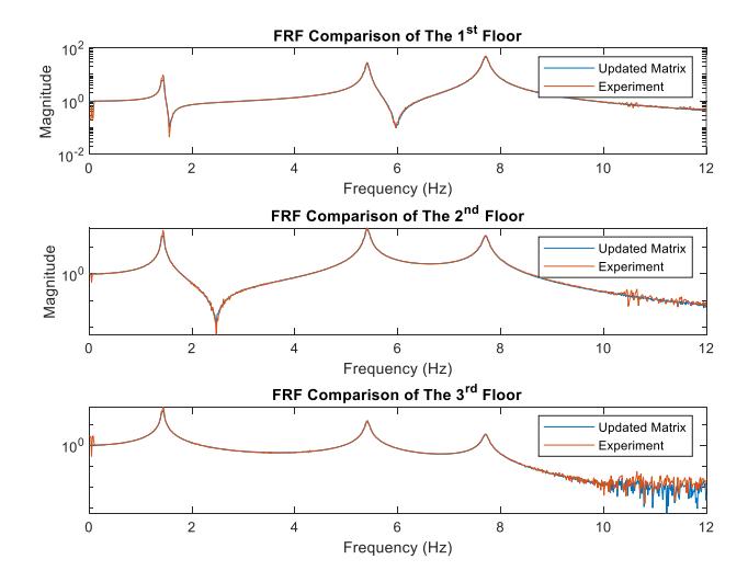
Figure 2 FRF comparison between the updated finite element model and the experiment result.
Control System Design
Linear Quadratic Regulator (LQR)
The optimal control force from linear control theory can be stated as in Eq. (7):
\[\mathbf{u}(t) = -\mathbf{G}\mathbf{Z}(t) \tag{7}\]
The G matrix is known as the gain matrix obtained from the optimal control algorithm. The optimal control force is determined by minimizing performance index J considering the system constraints. The form of performance that is usually chosen is the quadratic form of the responses and forces shown in Eq. (8):
\[J = \frac{1}{2} \int_{t_0}^{t_f} [\mathbf{Z}(t)^T \mathbf{Q} \mathbf{Z}(t) + \mathbf{u}(t)^T \mathbf{R} \mathbf{u}(t)] dt\] (8)
where \(\mathbf{Q}\) is the weight matrix for system response and \(\mathbf{R}\) is the weight matrix for the control force. The values of \(\mathbf{Q}\) and \(\mathbf{R}\) are chosen in such a way that good response reductions and an efficient control force are achieved. The weight matrices used in this study were:
\[\text{[rumus tidak dapat ditampilkan dengan baik — lihat PDF asli]}\]
Determination of the optimal control can be viewed as an optimization problem. The solution to the optimal control force can be stated as follows:
\[\mathbf{u}(t) = -\mathbf{G}\mathbf{Z}(t) = -\mathbf{R}^{-1}\mathbf{B}_{\mathbf{u}}^{\mathbf{T}}\mathbf{P}(t)\mathbf{Z}(t)\] (9)
The P(t) matrix, referred to as the Riccati matrix, can be determined by solving Eq. (10):
\[PA + A^{T}P - PB_{u}R^{-1}B_{u}^{T}P + Q = 0\] (10)
Thus, the gain matrix used for this study was:
\[\mathbf{G} = 10^4 [-0.113 \quad -3.462 \quad 2.178 \quad 0.019 \quad -0.045 \quad 0.1197]\]
Artificial Neural Network (ANN) based Controller
In conventional methodologies, the Linear Quadratic Regulator (LQR) determines the control force through full state feedback, which is rarely feasible in practical scenarios. Consequently, an alternative function or model is needed to replace the LQR. State of the art methods for time series prediction in recent years use recurrent neural network (RNN) architectures. However, those structures are more complex and computationally more expensive compared to a basic neural network architecture like a multilayered perceptron. Thus, by following recent research conducted by Pei-Ching Chen et al. [2], a model that is simpler than RNN, based on autoregression with exogenous input (ARX), was chosen in this study. The ARX model represents a neural network architecture where observations from previous time-steps are employed to forecast the current value. The ARX network can be formulated as follows:
\[u(t) = f\begin{pmatrix} \mathbf{u}(t-1), & \cdots & , \mathbf{u}(t-d_u) \\ \ddot{\mathbf{x}}(t), & \cdots & , \ddot{\mathbf{x}}(t-d) \end{pmatrix}\] (11)
The ARX model utilizes an open-loop method during the training phase, akin to that of a multilayer perceptron and uses a closed-loop model when implemented as a controller, as illustrated in Figure 3.
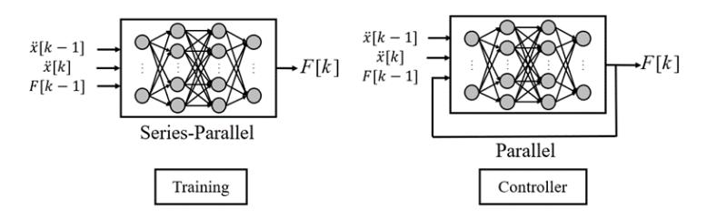
Figure 3 Autoregressive exogenous model.
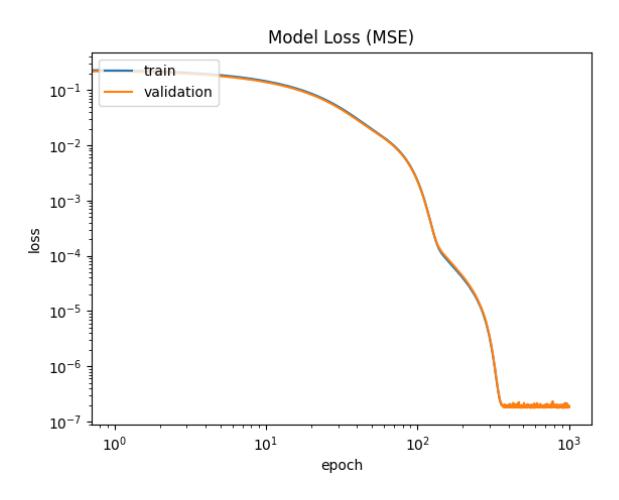
The ARX architecture chosen for this study was 7 × 20 × 20 × 20 × 1, where the inputs were two timesteps of acceleration on each floor and the control force at t-1. The inputs were normalized to ±1 and the neural network was trained using responses and force of the structure with LQR experiencing a random earthquake with 0.4 m/s2 peak acceleration. The parameters for training the neural network were:
- 1. All hidden layer's activation function = linear
- 2. Data splitting = 70:10:10 (training, validation, test)
- 3. Epoch = 1000
- 4. Initial learning rate = 0.00001
- 5. Loss function = mean squared error
- 6. Optimizer = Adam
- 7. Batch size = 128
The training process lasted less than an hour.
Training process of the ARX model.
Fuzzy Logic (FL) based Controller
Fuzzy set theory can be used to deal with uncertain phenomena in real-world applications. The theory enables objects to have any degrees of membership within a set. Fuzzy logic theory can be implemented in a controller to determine control forces.
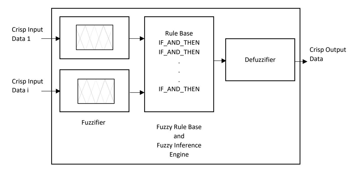
Fuzzy logic controller components.
The components of the fuzzy logic controller are: a fuzzifier (the measured inputs in the control process will be converted into linguistic value based on the membership functions), fuzzy rules (the collection of the control rules), a fuzzy inference engine (the unit to infer the control action from given inputs), and a defuzzifier (the inferred fuzzy control action will be converted to control value).
Developing a Fuzzy Logic Controller (FLC) typically demands specialized expertise. Thus, a metaheuristic algorithm can be used to help tuning the fuzzy logic controller. There are various metaheuristics algorithms, including genetic algorithm (GA) [12], Particle Swarm Optimization (PSO) [13] and Symbiotic Algorithm Search (SOS). SOS, developed by Cheng and Prayogo [16], is a recent metaheuristic algorithm and has been shown to perform relatively well compared to other similar algorithms and is simple to implement. Consequently, the SOS algorithm was selected for this study.
The SOS algorithm is a metaheuristic algorithm inspired by symbiosis between organisms to solve optimization problems. It consists of three phases (behaviours), i.e., the mutualism phase, the commensalism phase, and the parasitism phase. The mutualism phase modifies two candidate solutions based on the difference between the currently best solution and the difference between those two candidates. The commensalism modifies a candidate solution according to the difference between the currently best solution and the other candidate (organism). Lastly, the parasitism phase modifies an existing candidate solution randomly to enable the exploration of different regions from the solution field.
The inputs for the fuzzy logic controller in this study were acceleration of the top floor for time t, t-1, and control force for t-1 \((\ddot{x}_3(t), \ddot{x}_3(t-1), u(t-1))\). The fuzzifier consists of a membership function bounded in [-1,1] with five subsets (LN = Large Negative; N = Negative; Z = zero; P = Positive; LP = Large Positive) implemented for the three inputs.
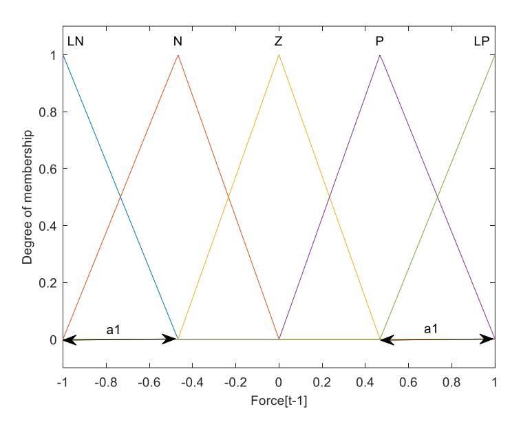
Figure 6 Membership function for control force [t-1].
There are several fuzzy inference systems, such as Mamdani [14] and Sugeno [15]. Mamdani's system possesses rule bases that are more intuitive and easier to comprehend, making them ideal for expert system applications. On the other hand, Sugeno's system is computationally more efficient and more suitable for control and optimization techniques. Therefore, Sugeno's system was chosen for this study.
Sugeno's inference system's output for each rule consists of multiplication of the rule weight and the linear function \(z_i\) of the corresponding output rules. It can be represented as in Eq. (12):
\[z_i = b_i \ddot{x}_3(t-1) + c_i \ddot{x}_3(t) + d_i u(t-1) + e_i\] (12)
The parameters \(b_i, c_i, d_i\), the normalization factor for the inputs, and parameter \(a_1\) in Figure 6 were optimized using SOS. Parameters \(a_2\) and \(a_3\) for input \(\ddot{x_3}(t)\) and \(\ddot{x_3}(t-1)\), respectively were treated the same.
The objective function used for SOS was in Eq. (13):
\[F_{obj} = min\left(\frac{\max(x_{3,fuzzy})}{\max(x_{3,uncontrolled})}\sqrt{\frac{1}{N}\sum_{i=1}^{N}(u_{fuzzy,i} - u_{LQR,i})^2}\right)\](13)
where \(x_{3,fuzzy}\) and \(x_{3,uncontrolled}\), represent the absolute acceleration of the third (top) floor for a structure with fuzzy controller and without active mass damper, respectively. Meanwhile, \(u_{fuzzy}\) and \(u_{LQR}\) are the control forces generated by FLC and LQR. The parameters of SOS were 10 organisms and 20 iterations. The optimization process lasted about 6 hours.
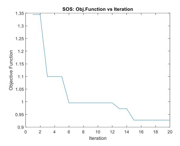
Figure 7 Optimization process of the FLC model's parameters.
Numerical Result and Discussion
Time Domain
The performances of the Al-based controllers were assessed by subjecting the structure to eight different earthquakes, as listed in Table 2. Particularly for the Kobe earthquake, the dominant frequency is close to the natural frequency of the structure's first mode. Thus, the response of the structure due to the Kobe earthquake will generally be greater than for the other earthquakes. The earthquakes were normalized to have a peak with 0.4 m/s<sup>2</sup> and the simulations were run using a 200 Hz sampling rate. Most earthquakes have a frequency of less than 20 Hz. Thus, the chosen sampling rate was considered adequate to capture the majority of earthquake frequencies. Additionally, the sampling rate also fulfilled Nyquist's criteria, which states that the sampling frequency must be more than twice the highest frequency of the signal captured.
Table 2 Earthquakes used in the study.
| Earthquake | Dominant Frequency [Hz] |
|---|---|
| El Centro | 1.47 |
| Chi-Chi | 1.32 |
| Chuetsu Oki | 0.70 |
| Kobe | 1.43 |
| Kumamoto | 4.89 |
| Montenegro | 1.78 |
| Parkfield | 1.66 |
| Darfield | 0.71 |
Seismic performance of the structure can be measured in various ways, ranging from drift ratio to the hysteretic curve, which is only applicable for a nonlinear model [18]. In this study, a linear analysis was conducted, and five performance indices were used in the numerical and experimental simulation. Four of the five performance indices were adopted from Dyke \(et\ al.\) [19] with performance 4 (\(I_4\)) as an addition. The performance indices were:
1. Relative displacement \(J_1 = \max_{t,i} \left(\frac{|x_t(t)|}{x_{max,unc}}\right) \tag{14}\)
2. Inter-story drift
\[J_2 = \max_{t,i} \left( \frac{|d_i(t)/h_i|}{(d/h)_{max,unc}} \right)\] (15)
3. Peak acceleration
\[J_3 = \max_{t,i} \left( \frac{|\ddot{x}_{ai}(t)|}{\ddot{x}_{aimax,unc}} \right) \tag{16}\]
4. Overall acceleration
\[J_4 = \max_{i} \left( \frac{RMS(\ddot{x}_{ai}(t))}{RMS(\ddot{x}_{ai,unc}(t))} \right)\] (17)
5. Control forces
\[J_5 = \max_{t \in \mathcal{X}} \left( \frac{|u(t)|}{W} \right) \tag{18}\] where \(x_i(t)\) is the relative displacement of the \(i^{\text{th}}\) floor during the excitation; \(x_{max,unc}\) is the maximum displacement of the uncontrolled structure; \(d_i(t)/h_i\) is the drift ratio of the \(i^{\text{th}}\) floor during excitation; \((d/h)_{max,unc}\) is the drift ratio of the \(i^{\text{th}}\) floor of the uncontrolled structure; \(\ddot{x}_{ai}(t)\) is the absolute acceleration of the \(i^{\text{th}}\) floor; \(\ddot{x}_{ai,unc}(t)\) is the absolute acceleration of the \(i^{\text{th}}\) floor of the uncontrolled structure; u(t) is the control force of AMD; and W is the weight of the structure
Tables 3 and 4 and list the performance indices for the fuzzy logic controller and the ANN-based controller, respectively. The tables show that the ANN-based controller generally reduced the structure response by 27.6% (the average value of \(J_1\)-\(J_4\)) better than the FL-based controller. On the other hand, the ANN-based controller needed 26.5% more force than the FL-based controller.
| Table 3 | Seismic control | performance | of ANN-based | AMD in | numerical study. |
|---|
| Earthquake | J1 | J2 | J3 | J4 | J5 |
|---|---|---|---|---|---|
| El Centro | 0.496 | 0.441 | 0.573 | 0.298 | 0.012 |
| Chi-Chi | 0.708 | 0.692 | 0.689 | 0.290 | 0.008 |
| Chuetsu Oki | 0.634 | 0.604 | 0.450 | 0.451 | 0.013 |
| Kobe | 0.642 | 0.611 | 0.551 | 0.223 | 0.019 |
| Kumamoto | 0.603 | 0.540 | 0.516 | 0.429 | 0.013 |
| Montenegro | 0.506 | 0.516 | 0.449 | 0.308 | 0.014 |
| Parkfield | 0.737 | 0.731 | 0.760 | 0.318 | 0.011 |
| Darfield | 0.620 | 0.588 | 0.731 | 0.406 | 0.008 |
| Average | 0.618 | 0.590 | 0.590 | 0.340 | 0.012 |
Table 4 Seismic control performance of FL-based AMD in numerical study.
| Earthquake | \(J_1\) | \(J_2\) | \(J_3\) | \(J_4\) | \(J_5\) |
|---|---|---|---|---|---|
| El Centro | 0.515 | 0.563 | 0.823 | 0.366 | 0.009 |
| Chi-Chi | 0.850 | 0.830 | 0.842 | 0.459 | 0.009 |
| Chuetsu Oki | 0.737 | 0.745 | 0.741 | 0.585 | 0.012 |
| Kobe | 0.873 | 0.874 | 0.910 | 0.737 | 0.012 |
| Kumamoto | 0.749 | 0.705 | 0.730 | 0.707 | 0.007 |
| Montenegro | 0.844 | 0.845 | 0.879 | 0.571 | 0.012 |
| Parkfield | 0.938 | 0.948 | 0.871 | 0.400 | 0.012 |
| Darfield | 0.855 | 0.874 | 0.891 | 0.503 | 0.007 |
| Average | 0.795 | 0.798 | 0.836 | 0.541 | 0.010 |
With significantly less training time, the ANN-based controller performed better than the FL-based controller. Despite its low effectiveness, FLC still reduced the structure's responses with smaller forces than the ANN controller.
Frequency Domain
The responses in the time domain can be converted to the frequency domain to investigate the changes in the dynamic properties of the structure. Figure 8 shows the comparison of FRFs between the uncontrolled, ANN-controlled, and fuzzy-controlled structures.
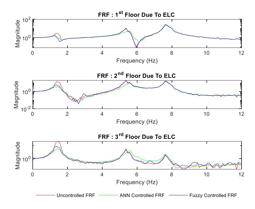
Frequency response function comparison for ELC.
The changes in natural frequency shown in Table 5 are small compared to changes in the damping ratio of the structure shown in Table 6. Both models gave an increase in damping ratio, with a significant impact in the first mode of the structure followed by its second and third modes. In the ANN-based controller, increasing demand led to an increase in damping ratio. An abnormality can be seen in FLC, where the damping ratio increase in response to the Kobe earthquake, with the largest demand due to resonance, was the smallest. Therefore, the ANN-based controller for AMD provides more consistency in reducing structure responses.
Table 5 Natural frequency of the controlled structure.
| Uncontrolled | ANN | Fuzzy | |||||||
|---|---|---|---|---|---|---|---|---|---|
| EQ | f1[Hz] | f2[Hz] | f3[Hz] | f1[Hz] | f2[Hz] | f3[Hz] | f1[Hz] | f2[Hz] | f3[Hz] |
| El Centro | 1.41 | 5.53 | 7.66 | 1.40 | 5.38 | 7.66 | |||
| Chi-Chi | 1.40 | 5.51 | 7.71 | 1.37 | 5.41 | 7.70 | |||
| Chuetsu Oki | 1.39 | 5.52 | 7.68 | 1.38 | 5.38 | 7.69 | |||
| Kobe | 1.39 | 5.53 | 7.71 | 1.43 | 5.40 | 7.70 | |||
| Kumamoto | 1.43 | 5.41 | 7.71 | 1.40 | 5.52 | 7.70 | 1.38 | 5.39 | 7.70 |
| Montenegro | 1.40 | 5.40 | 7.67 | 1.40 | 5.40 | 7.67 | |||
| Parkfield | 1.41 | 5.53 | 7.70 | 1.36 | 5.40 | 7.70 | |||
| Darfield | 1.40 | 5.52 | 7.71 | 1.37 | 5.40 | 7.71 | |||
| Average | 1.40 | 5.51 | 7.69 | 1.39 | 5.40 | 7.69 | |||
Table 6 Damping ratio of the controlled structure.
| Uncontrolled | ANN | Fuzzy | |||||||
|---|---|---|---|---|---|---|---|---|---|
| EQ | ζ1[%] | ζ2[%] | ζ3[%] | ζ1[%] | ζ2[%] | ζ3[%] | ζ1[%] | ζ2[%] | ζ3[%] |
| El Centro | 6.47 | 1.96 | 1.42 | 3.45 | 1.55 | 1.17 | |||
| Chi-Chi | 5.08 | 2.07 | 0.85 | 3.41 | 0.90 | 0.71 | |||
| Chuetsu Oki | 5.10 | 2.02 | 1.16 | 3.82 | 1.11 | 1.03 | |||
| Kobe | 6.71 | 1.82 | 0.54 | 1.51 | 0.85 | 0.23 | |||
| Kumamoto | 0.92 | 0.51 | 0.57 | 6.64 | 2.24 | 0.89 | 3.55 | 1.25 | 0.67 |
| Montenegro | 5.26 | 2.03 | 1.10 | 4.43 | 0.71 | 0.97 | |||
| Parkfield | 4.35 | 1.41 | 0.45 | 2.06 | 0.61 | 0.19 | |||
| Darfield | 6.44 | 2.21 | 0.77 | 3.84 | 1.03 | 0.62 | |||
| Average | 5.76 | 1.97 | 0.90 | 3.26 | 1.00 | 0.70 | |||
In the design phase, the FL controller needed considerably more time to optimize its parameters than the ANN controller (6 hours compared to less than 1 hour). In the numerical simulation, ANN also gave better performance and consistency than FL. Although the FLC's performance may be further improved by extending and improving the optimizing process, the FLC will need additional resources and time to an already long process. Correspondingly, training ANN is more straightforward and quicker than FLC. Therefore, the ANN-based controller was chosen as the best AI-based controller for an AMD and only the ANN-based controller was implemented in the experimental study.
Experimental Result and Discussion
Experimental Setup
The experiment was conducted in a small-scale laboratory in the National Center for Research on Earthquake Engineering (NCREE) in Taipei, Taiwan. The experiment specimen was a three-story building with the AMD installed on the top floor, as shown in Figure 9.
Experimental setup.
The AMD consisted of electric servo motors, driving screws, slide rails, and a mass slider. The shaking table was driven by a servo-hydraulic actuator with a maximum output force of 15 kN and a maximum stroke of ±125 mm. Five SDI highresolution MEMS accelerometers were used with the maximum capability ±25 m/s2 to measure the acceleration. The accelerometers were installed on the shaking table, on each floor, and on the AMD.
The controllers were all constructed in MATLAB/Simulink to be able to control the hydraulic actuator and the AMD. The performance real-time target machine developed by Speedgoat shown in Figure 10 was used. The performance realtime target machine is a real-time test system that supports Simulink and Simulink Real-Time. The system modules provided by Simulink Real-Time were connected to the host computer via TCP/IP network communication protocol I/O terminals that compiled the MATLAB/Simulink code into C language and loaded it onto the host to calculate and control the AMD.
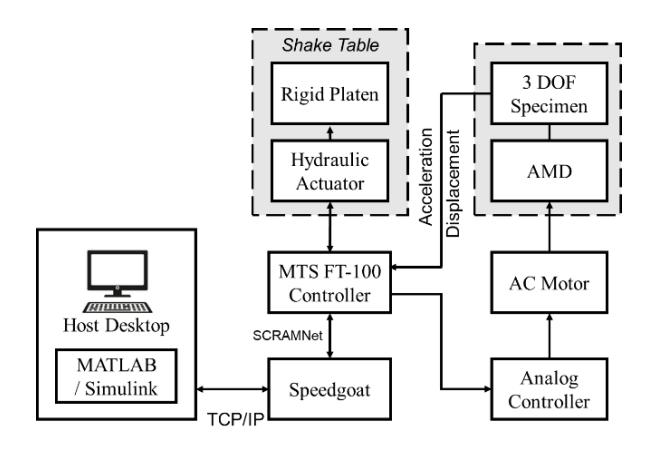
Hardware and software setup in the experimental study.
In addition, SCRAMNet optical fiber shared memory was used to enable the performance of the real-time target machine and MTS FT- 100 to share memory and data. Therefore, the host could control the hydraulic actuator and electric motor AMD at the same time during the experiment.
Result and Discussion
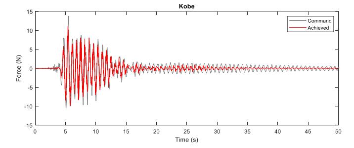
The performance of the ANN-based controller from the experimental study can be seen in Table 7. The performance in the experimental study tended to be lower than in the numerical study. The main reason was that the force generated by the AMD in the experiment was unable to match the desired force by the controller, as shown in Figure 11.
| Earthquake | J1 | J2 | J3 | J4 | J5 |
|---|---|---|---|---|---|
| El Centro | 0.490 | 0.471 | 0.523 | 0.368 | 0.009 |
| Chi-Chi | 0.697 | 0.638 | 0.660 | 0.391 | 0.006 |
| Chuetsu Oki | 0.733 | 0.713 | 0.709 | 0.485 | 0.012 |
| Kobe | 0.676 | 0.681 | 0.593 | 0.304 | 0.015 |
| Kumamoto | 0.675 | 0.693 | 0.712 | 0.529 | 0.010 |
| Montenegro | 0.670 | 0.659 | 0.640 | 0.425 | 0.014 |
| Parkfield | 0.944 | 0.922 | 0.947 | 0.421 | 0.009 |
| Darfield | 0.724 | 0.705 | 0.773 | 0.465 | 0.005 |
Table 7 Seismic control performance of ANN-based AMD in the experimental study.
Average 0.701 0.685 0.695 0.424 0.010
Command and achieved force for the Kobe Earthquake with 0.4 m/s2 PGA.
Despite the differences, the ANN-based controller still showed the ability to reduce the structure's responses with an average reduced performance of 18% and a 19% smaller force compared to the numerical results.
Conclusions
This study investigated two AI models, namely, artificial neural network (ANN) and fuzzy logic (FLC), for the controller of an active mass damper (AMD). In the design phase, the elapsed time for training ANN was considerably less than that for optimizing FLC. It was also evident that ANN provides better performance, as shown in the performance indices value from the numerical study. The ANN-based AMD also demonstrated better consistency, as shown in providing the highest damping ratio on the structure when excited with the highest demand earthquake, the Kobe earthquake. In contrast, the FL-based AMD provides the smallest damping ratio during the same earthquake. Therefore, the results for this specific structure in this study showed that ANN is a more straightforward AI model to be implemented as an AMD controller compared to FLC. Furthermore, this study successfully implemented and validated the ANN-based AMD through experimental studies using a prototype-sized three-story building.
Acknowledgements
Financial support for this study was provided through Institute for Research and Community Services (LPPM) and the Faculty of Civil and Environment Engineering, Institut Teknologi Bandung, Indonesia.
Compliance with ethics guidelines
The authors declare that they have no conflict of interest or financial conflicts to disclose.
This article does not contain any studies with human or animal subjects performed by any of the authors.