
Introduction
The energy losses in the distribution networks of a power system account for a high rate of power loss in the whole system [1]. These losses challenge researchers and power system operators to find solutions [2]. Currently, the installation of onsite distributed generators (ODGs) in distribution power systems (DPSs) is encouraged, which can improve the technical and economic characteristics of the system [3]. In this study, the combination of wind-based distributed generators (WDG) and solar photovoltaic distributed generators (PVDGs) was implemented for one operating day with the purpose of cutting power losses.
Previous studies have implemented the installation of ODGs in DPS for two main purposes. The study [4] concentrated on distributed generation allocation to minimize power system losses and balance power generation and demand by applying the Equilibrium Optimization Algorithm (EOA). The studies [6-7] applied the Artificial Ecosystem Optimization (AEO) algorithm for power loss reduction in IEEE-33 bus and IEEE-69 bus DPSs. In study [8], the Sine Cosine Algorithm (SCA) could optimize the placement of ODGs for achieving different objectives, including power loss mitigation and voltage profile improvement. The above-mentioned studies considered ODGs without considering the fuel and generator types, while others indicated clear types. The studies [9-15] optimized placement-only capacitor banks (CBs) with reactive power generation by different algorithms, such as the Moth Swarm Algorithm (MSA) [9], the Stochastic Programming (SP) approach [10], the Bacterial Foraging Optimization Algorithm (BFOA) [11], the Flower Pollination Algorithm (FPA) [12], the Gravitational Search Algorithm (GSA) [13], and the Teaching Learning Based Optimization (TLBO) algorithm [14], and the Whale Optimization Algorithm (WOA) [15]. These studies focused on standard IEEE DPSs with 33, 69 and 85 nodes and reached loss reduction and voltage improvement.
Nowadays, renewable energy sources-based distributed generators, WDGs and PVDGs are more popular for reaching these purposes. The studies [16-17] used the same PVDG in DPSs but different algorithms, Coulomb-Franklin's Algorithm (CFA) [16] and a biogeography-based optimization (BBO) [17]. The study [18] applied PVDGs and unbalanced DPSs. In contrast, the studies [19-21] used WDGs for different purposes and DPSs. Other studies [22-25] applied reconfiguration for DPSs. The studies [26-28] applied both PVDGs and WDGs to deal with a similar problem. In general, these studies generated active and reactive power to grid instead of using that from conventional power sources to reduce the current. Current reduction is one of the most effective ways to reduce losses and improve the voltage [29-30].
In this paper, both PVDGs and WDGs were optimally placed for an IEEE-85 bus DPS. Unlike the above-mentioned studies, this research used the Global Wind Atlas [31] and the Global Solar Atlas [32] for collecting wind speed and solar radiation for one operating day. Besides, a novel meta-heuristic algorithm, the Wild Horse Optimizer Algorithm (WHOA) [33], was applied. WHOA was run on several sets of test functions, including CEC2017 and CEC2019. For comparison, the Archimedes Optimization Algorithm (AOA) [34] and transient search optimization (TSO) [35] were also applied to the considered problem to revalidate the real effectiveness of WHOA. The results revealed that the proposed algorithm produced highly competitive results compared to the other algorithms.
The main contributions of this study can be summed up in the following points:
- 1. Evaluate the effectiveness of PVDGs and WDGs over 24 hours on an IEEE 85-node DPS as a real system.
- 2. Reduce power losses and improve the voltage of the system effectively.
- 3. Demonstrate the superiority of WHOA when compared with other state-of-the-art meta-heuristic algorithms, such as AOA and TSO, in terms of different criteria.
- 4. Recommend a plan of placing renewable energies-based generators on DPSs.
Problem Description
Main Objective Function
The study focused on power loss reduction for the considered networks over twenty-four hours of one day as follows:
Reduce \[\sum_{b=1}^{Br} APL_b = 3\sum_{b=1}^{Br} \sum_{h=1}^{24} I_{bh}^2 R_b\] (1)
where \(APL_b\) is the active power loss in the b-th branch of the given DPS with b = 1, ..., Br; Br is the number of branches in the DPS; \(I_{bh}\) is the operating current of the b-th branch at the h-th hour; and \(R_b\) is the resistance of the b-th branch.
Related Constraints
The operation voltage constraint. This constraint considers the operating limits of the voltage of the nodes as follows:
\[V_n^l \le V_n \le V_n^h; n = 1, \dots, N \tag{2}\] where \(V_n^l\) and \(V_n^h\) are the lowest and the highest values of the operating voltage at node n; \(V_n\) is the actual voltage measured at node n; and N is the quantity of nodes in the given DPS.
Operational constraint of CBs, PVDGs and WDGs. These electric components must be within the upper and lower generation limits, as shown in the expressions below:
\[QC_c^l \le QC_c \le QC_c^h; c = 1, \dots, N_{CBS}\] \[\tag{3}\]
\[PVP_{nv}^{l} \le PVP_{nv} \le PVP_{nv}^{h} : pv = 1, \dots, N_{PVS}\] \[\tag{4}\]
\[WP_w^l \le WP_w \le WP_w^h; w = 1, ..., N_{WS}\] (5)
where \(QC_c^l\) and \(QC_c^h\) are the lowest and highest reactive power supplied by the c-th bank; \(PVP_{pv}^l\) and \(PVP_{pv}^h\) are the lowest and highest generation of the pv-th PVDG; \(WP_w^l\) and \(WP_w^h\) are the lowest and highest generation values of the w-th WDG; \(QC_c\), \(PVP_{pv}\) and \(WP_w\) are the generation values of the c-th CB, the pv-th PVDG and the w-th WDG; and \(N_{CBS}\), \(N_{PVS}\) and \(N_{WS}\) are the number of CBs, PVDGs and WDGs.
Branch operational current constraints: The operating current of all branches should satisfy the following inequality:
\[I_b \le I_b^{DCS}; b = 1, \dots, Br \tag{6}\]
wher, is the working current on branch b, and is the maximum current of branch b.
Placement location constraint of PVDGs and WDGs. In DPSs, a transformer is located at node 1, so PVDGs and WDGs can be located from node 2 to node N, as expressed by:
\[2 \le PVL_{pv} \le N \tag{7}\]
\[2 \le WL_w \le N \tag{8}\] where, and are the location of the pv-th PVDG and the w-th WDG, respectively.
Applied Method
Wild Horse Optimization Algorithm
The Wild Horse Optimizer algorithm (WHOA) [33] is a metaheuristic optimization algorithm inspired by the behavior of wild horses and their grazing and herding patterns. By imitating these behaviors, the algorithm can provide an exceptional balance in both the exploration and exploitation phases of the optimization process by mimicking wild horses' grazing and herding patterns. WHOA has been tested on various benchmark problems and has shown promising results, making it a competitive optimization tool for solving complex problems. Similar to the two previously applied methods above, the critical executions regarding the update procedure of WHOA is presented below:
\[W_{k,g}^{new} = \begin{cases} 2 \times AI \times cos(2\pi \times UR \times AI) \times (LD_g + W_{k,g}) + LD_g, & RnD > 0.13 \\ \frac{W_{p,t} + W_{q,f}}{2}, & otherwise \end{cases}\](9)
In the equation, , is the new solution k in group g, with k = 1, 2…, Pg and Pg is the population size of group g. Note that the population number of all groups is equal to the population size (Pz) required by WHOA at the beginning of the optimization process. , is solution p in group t and , is the current solution q in group f. the best solution of group g. is a random value between 0 and 1. UR is the unified random factor between -2 and 2. is the adaptability indicator, which is obtained as follows:
\[AI = RnD \ominus IX + RnD \ominus (\sim IX) \tag{10}\] with
\[IX = (P == 0) \tag{11}\]
\[P = RnD < TDR \tag{12}\]
Note that, in Eq. (9), the indexes of g, t, and f are different from each other. Similarly, the indexes of k, p, and q are also not the same.
Numerical Results
Figure 1 shows a single-line diagram of the 85-bus DPS [11]. This system consists of 85 buses and 84 distribution lines. The system's total real power and reactive power demand are 2570.28 kW and 2621.936 kVAR, respectively. The base values per unit (p.u.) are Sbase = 100 MVA and Vbase = 11 kV. The power loss in the base case is 315.3 kW.
The following sections present the analysis of the results obtained using various algorithms applied to the 85-bus IEEE system:
Case 1: Optimizing location and size of CBs in one hour
Case 2: Optimizing location and size of ODGs in one hour
Case 3: Optimizing location and size of one WDG and one PVDG in twenty-four hours
Case 4.1: Using the determined WDG and PVDG in Case 3 and optimizing one more WDG and one more PVDG in twentyfour hours
Case 4.2: Optimizing two WDGs and two PVDGs simultaneously in twenty-four hours
Configuration of the IEEE 85 bus.
Case 1: Optimal Placement of Three CBs
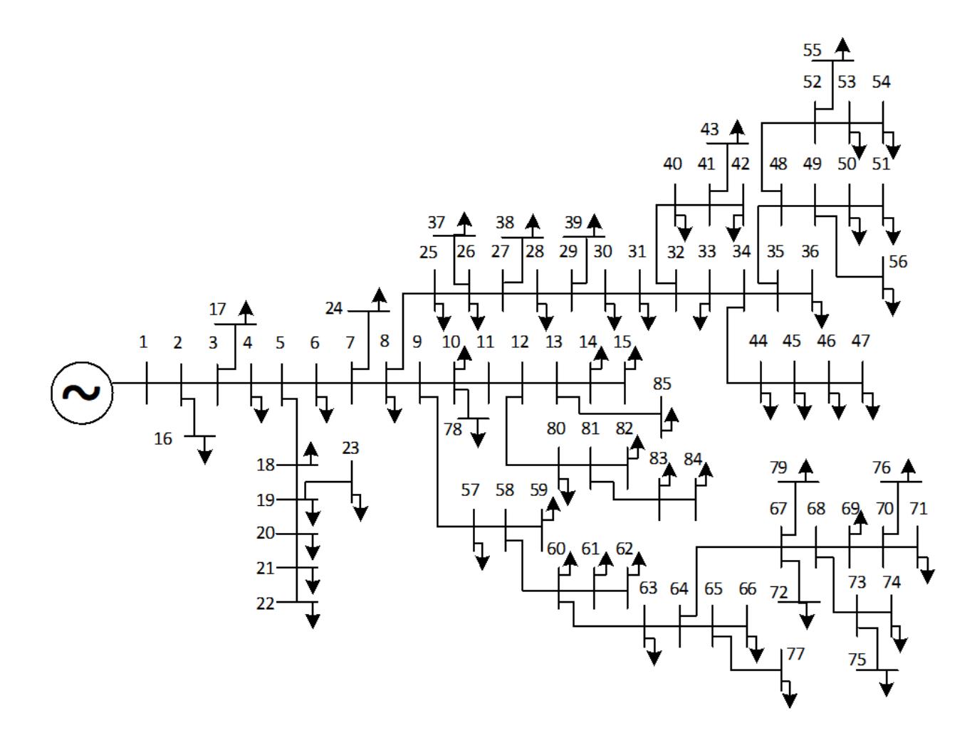
In this section, several algorithms were applied to optimize the location and size of CBs in the grid. These algorithms were WHOA, AOA, and TSO. These techniques aim to determine the optimal locations and sizes of CBs to achieve reduced power loss in the grid. The methods were run for fifty trials by setting Pz and ITmax to 20 and 400. The results are depicted in Figure 2. This figure reveals that the outcomes of the fifty runs obtained by the WHOA method consistently fell within the range of 150.85 kW to 154.99 kW, TSO exhibited values ranging from 156.16 kW to 165.65 kW, and notably, AOA concentrated its values between 166.53 kW and 187.84 kW. This indicates that the WHOA method outperformed both TSO and AOA.
Furthermore, the minimum result obtained from the fifty runs using the WHOA method was 150.85 kW, superior to that of TSO (152.13 kW) and AOA (153.86 kW). Table 1 presents the overall power loss, optimal locations and sizes of CBs obtained by various techniques, including WHOA, AOA, TSO, BFOA [11], FPA [12], and CFA [16]. Among the methods, WHOA achieved the lowest power loss after compensation, at 150.85 kW. The optimal positions of CBs in the grid were 9, 34, and 67, with corresponding capacitance values of 1074.39 kVar, 672.40 kVar, and 527.42 kVar, respectively. Additionally, the installation of CBs also led to an improvement in the voltage profile of the system, which is easily observable in Figure 3. The voltage profile after capacitor installation was significantly higher than the profile without their installation.
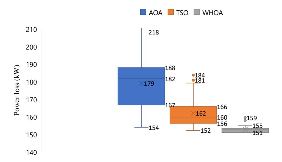
Figure 2 Summary of 50 runs obtained by the three applied algorithms for Case 1.
Table 1 The results of Case 1 between the applied method and other methods from previous studies.
| Method | Bus, size (kVar) | Total power loss (kW) |
|---|---|---|
| BFOA [11] | (9; 840.00), (34; 660.00), (60; 650.00) | 152.25 |
| FPA [12] | (8; 1200.00), (36; 600.00), (72; 600.00) | 151.81 |
| CFA [16] | (9; 200.00), (34, 600.00), (68, 450.00) | 151.10 |
| AOA | (8; 761.21), (48; 558.77), (63; 811.73) | 153.86 |
| TSO | (9; 921.50), (32; 818.88), (67; 565.21) | 152.13 |
| WHOA | (9; 1074.39), (34; 672.40), (67; 527.42) | 150.85 |
Figure 3 Voltage profile for Case 1.
Case 2: Optimal Placement of Three ODGs
WHOA, AOA and TSO were used to optimize the location and size of ODGs to minimize the power loss within the grid. The methods were run for fifty trials by setting the population and iteration number to 20 and 400, respectively. The obtained results are graphically represented in Figure 4. The plot demonstrates that WHOA obtained loss values in the range of 148.67 kW to 151.22 kW. TSO exhibited loss values ranging from 156.52 kW to 168.94 kW, while AOA concentrated its values between 158.27 kW and 172.39 kW. These findings highlight the superior performance of the WHOA method over both TSO and AOA.
Table 2 provides comprehensive information regarding the overall power loss and the optimal locations and sizes of ODGs obtained by WHOA, AOA, TSO, and CFA [16]. Notably, the WHOA method achieved the lowest power loss after compensation, with a measurement of 148.67 kW, which represents the most favorable outcome. The optimal grid installation positions were 9, 34, and 67, corresponding to capacitance values of 1094.60 kW, 675.52kW, and 524.14 kW, respectively. Furthermore, installing distributed generation also enhanced the voltage profile within the system, as visually illustrated in Figure 5. The voltage profile after the installation of distributed generation exhibited significantly higher values than the profile without their presence.
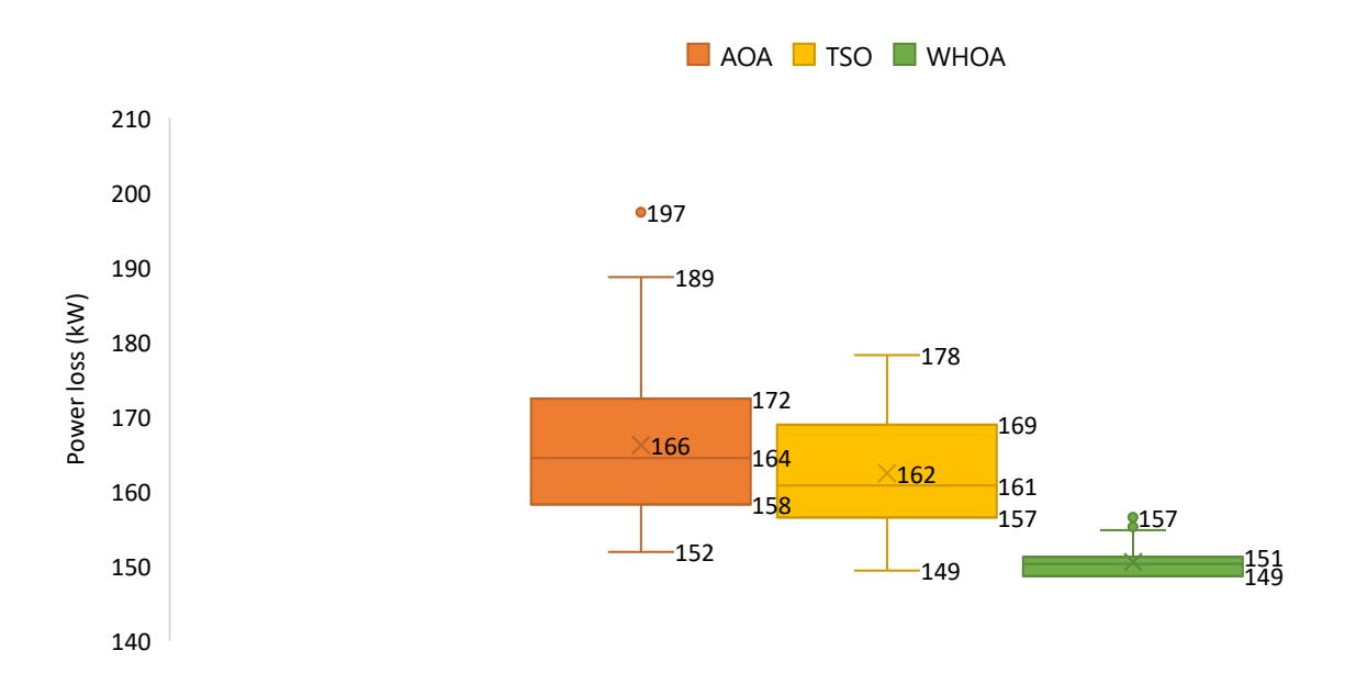
Summary of 50 runs obtained by three applied algorithms for Case 2.
Table 2 The results of Case 2 between the applied method and other methods from previous studies.
| Method | Bus; size (kW) | Total power loss (kW) |
|---|---|---|
| CFA [16] | (9; 1058.17), (34; 681.87), (67; 533.44) | 148.69 |
| AOA | (32; 846.46), (57; 958.16), (68; 305.60) | 151.88 |
| TSO | (9; 1271.09), (34; 713.45), (68; 322.76) | 149.42 |
| WHOA | (9; 1094.60), (34; 675.52), (67; 524.14) | 148.67 |
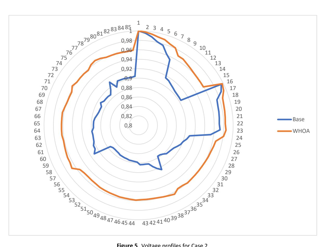
Figure 5 Voltage profiles for Case 2.
Case 3: Optimal Placement of One PVDG and One WDG
In this section, the three applied algorithms were run for optimizing one WDG and one PVDG in the IEEE 85-bus system, considering a period of twenty-four hours. The load factors over the hours are given in Figure 6. The total energy losses and the total energy demand of the base case before installing the ODGs were 3,880.5 kWh and 43,489.14 kWh. Thus, the energy from the grid must be equal to the sum of these values, equaling 47,369.67 kW. The energy loss, demand and supply of the grid are presented in Figure 7.
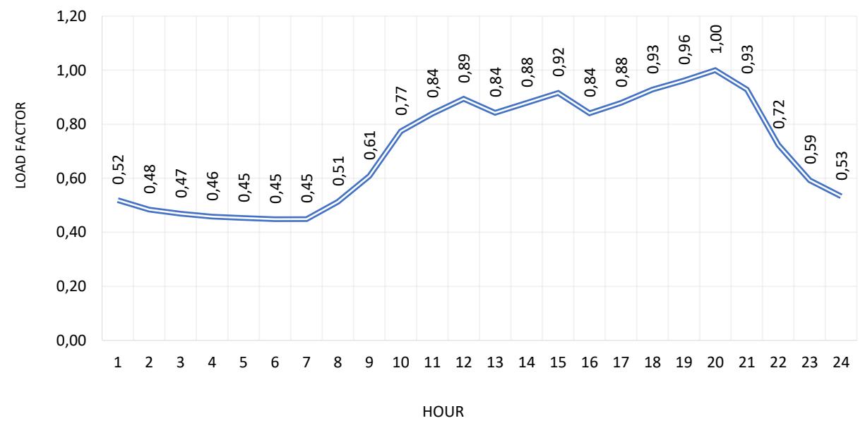
Figure 6 Power demand.
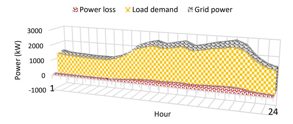
Graph of power loss, load demand, and grid power.
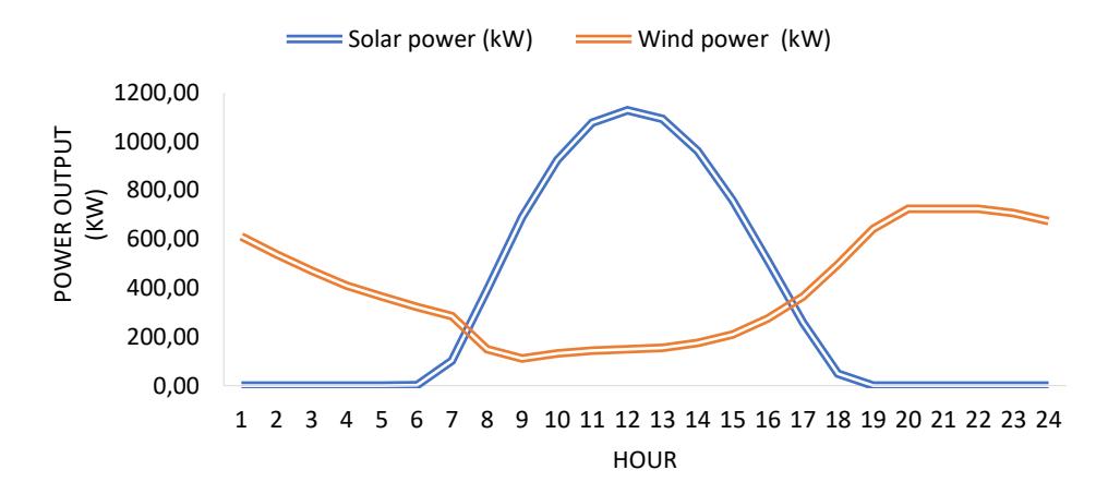
Based on the global solar data [31], at the location of 10.631237° and 106.719938°, the PVDG is classified as a mediumsized commercial system. The azimuth of the PVDG was set to the default value of 180º, while the tilt of the PVDG panels was adjusted to 12º. The installed capacity of the PVDG was 2000 kWpta (kilowatts peak to average). From the global wind data [32], at the exact location of 10.631237° and 106.719938°, the average wind speed was determined. The power output from both PVDG and WDG were calculated, as presented in Figure 8.
Graph of power loss, load demand, and grid power.
Case 4: Optimal Placement of Two PVDGs and Two WDGs
This section discusses two simulation scenarios regarding the optimal placement of two PVDGs and two WDGs, Case 4.1 and Case 4.2. The two cases used the same number of ODGs, but the placement plan was different. Case 4.1 assumed that one PVDG and one PVDG were optimally placed previously, and now one more PVDG and one more WDG were planned to be placed. Case 4.2 assumed that the power grid did not have any renewable distributed generators placed optimally previously. The results from Case 3 above were inherited for Case 4.1, while Case 4.2 performed a new simulation.
The WHOA algorithm was selected as an efficient method for solving the two cases. The results of the total power loss and grid power obtained from Case 4.1 and Case 4.2 were compared to those from the base case and Case 3 in Figure 9. Case 3, Case 4.1 and Case 4.2 could reach a smaller loss than the base case by 1963.4 kW, 2956.1 kW, and 3012.3 kW, respectively. Comparison between Case 4.1 and Case 4.2 indicates that Case 4.2 could reach a smaller loss of 56.2 kW. In addition, installing PVDGs and WDGs in the system also reduced the power received from the grid. In the base system, power received from the grid was 47369.7 kW. When increasing the number of ODGs, the power received from the grid could be reduced more. It was 27907.8 kW for Case 3, 9416.8 kW for Case 4.1, and 9360.6 kW for Case 4.2. Compared to the base case, Case 3 used less power from the grid by 41.09%, while Case 4.1 and Case 4.2 used less power from the grid by 80.12% and 80.24%.
As compared to Case 3 and Case 4.1, Case 4.2 used the least power from the grid. This was also the result of the power losses over 24 hours shown in Figure 10. The power loss from Case 4.2 was significantly smaller than that from Case 3 and Case 4.2 for hours 11 to 14 and hours 18 to 21. Case 4.2 also reached a smaller loss for other hours than Case 3 and Case 4.1.
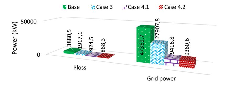
Power loss and grid power obtained for the study cases.
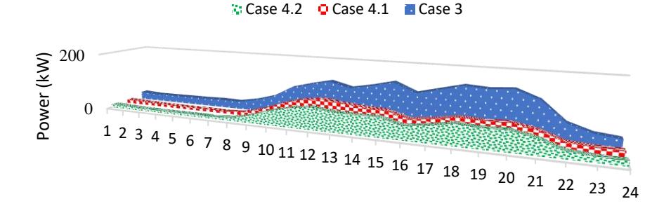
Power losses over 24 hours for Case 3, Case 4.1, and Case 4.2
Power over 24 hours in the study cases.
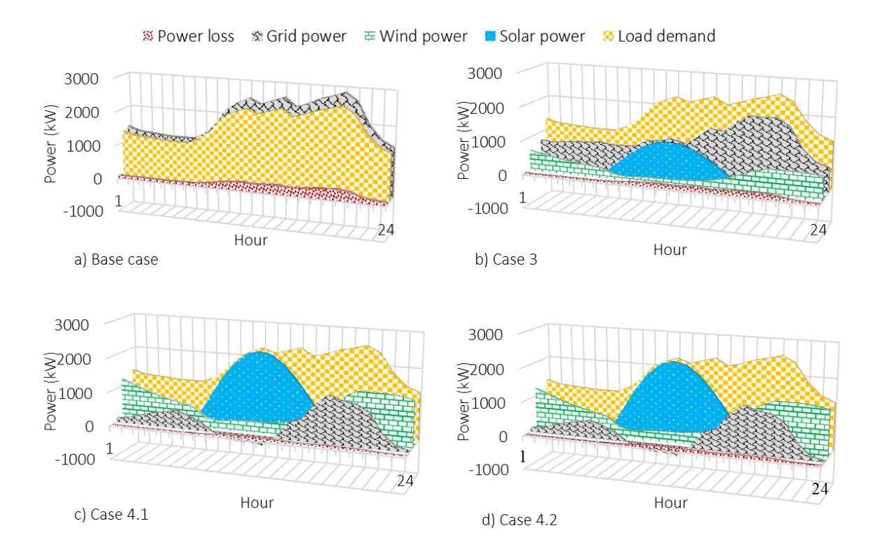
Figure 11 presents the load demand, power loss, grid power, and power output of the ODGs for the base case, Case 3, Case 4.1, and Case 4.2. The figure shows that Case 4.1 and Case 4.2 have the same shape, where we cannot find a difference, whereas the two cases are very different from Case 3. The base case is without PVDGs and WDGs, so the grid power is on top, and the loss can be clearly seen. The graphic results for Case 4.1 and Case 4.2 cannot indicate the advantage of the renewable energy installation plan; however, the loss reduction in the numerical result, 56.2 kW, can clarify the benefit of a specific plan. The simultaneous placement of two WDGs and two PVDGs was more effective than the respective placement, i.e., one PVDG and one WDG in Case 3 and then one PVDG and one WDG in Case 4.1.
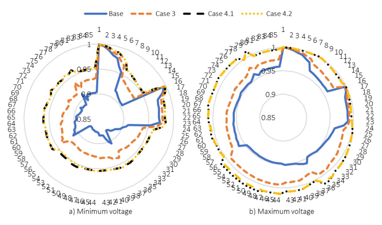
Figure 12 presents the minimum and maximum voltage of the nodes from the base case, Case 3, Case 4.1, and Case 4.2 over twenty-four hours. The base case had many nodes violating the voltage limits under 0.9 pu, while other cases could prevent violations. The minimum voltage of Case 3 was around 0.92, while that of Case 4.1 and Case 4.2 was around 0.95. The maximum voltage of Case 4.1 and Case 4.2 was greater than 1.0 and smaller than 1.05 pu as the voltage constraint. The base case and Case 3 had many nodes with the maximum voltage ranging from 0.95 to smaller than 1.0, while the base case had a small number of nodes, i.e., close to 1.0 pu. The result shows that the installation of PVDGs and WDGs is very useful for improving the voltage even though the initial purpose was the reduction of power loss.
The minimum and maximum voltage achieved in Case 3, Case 4.1, and Case 4.2
Conclusions
This study applied WHOA, AOA and TSO to determine optimal locations and sizes of CBs, PVDGs and WDGs in an IEEE 85-bus distribution power system. The results demonstrated the superiority of the WHOA algorithm over AOA and TSO in finding optimal solutions, outperforming other algorithms used in previous studies, such as BFOA [11], FPA [12], and CFA [16]. In Case 1, with the placement of three CBs, WHOA reached smaller loss values than AOA, TSO, BFOA [11], FPA [12], and CFA [16]. In Case 2, with the placement of three ODGs, WHOA achieved smaller loss values than AOA, TSO, and CFA [16]. In Case 3, Case 4.1 and Case 4.2, WHOA successfully found PVDGs and WDGs to get a reduced total loss over twenty-four hours. All constraints, especially the node voltage, were satisfied within the predetermined range. The placement of two PVDGs and two WDGs in Case 4.1 and Case 4.2 was superior to Case 3 in terms of power loss reduction and voltage improvement. Case 4.2 with the simultaneous placement of two PVDGs and two WDGs was superior to Case 4.1. Case 4.1 used the placement of one WDG and one PVDG of Case 3 and then placed one more PVDG and one more WDG. The results indicated that a predetermined plan of using a number of PVDGs and WDGs is very useful in reducing power loss and improving voltage.
Acknowledgement
This research was funded by Hanoi University of Science and Technology through project code T2023-PC-040.
Compliance with ethics guidelines
The authors declare that they have no conflict of interest or financial conflicts to disclose.
This article does not contain any studies with human or animal subjects performed by any of the authors.