
Introduction
Using renewable and sustainable alternative fuels for automotive engines is essential for reducing the dependence on depleting fossil fuels. The extensive consumption of conventional fuels like gasoline and diesel worsens the environmental problems and poses a threat to global energy security. Various alternative fuel options are available nowadays, which include ethanol, methanol, DME as a substitute for gasoline and diesel. These alternative fuel options have shown promise in reducing emissions and enhancing energy sustainability to the researchers (Kodancha et al., 2020; G. Singh et al., 2021; Bawase & Thipse, 2021; Kavathekar et al., 2021).
One of the promising alternate fuels for gasoline is ethanol, which offers various advantages over traditional gasoline. Ethanol possesses higher octane rating characteristics, enabling the use of a higher compression ratio, further enhancing the engine performance. Also, ethanol has inherent oxygen in its chemical structure that promotes cleaner and more efficient combustion, further leading to better fuel utilization and reduced emissions. These characteristics of ethanol fuel make it an environment-friendly option. Furthermore, ethanol can be produced by using corn, maize, sugarcane, broken grains, grass, etc. which are renewable in nature and abundant in the country like India. This renewable and localized approach enhances this fuel's prominence while also supporting the agriculture sector. In India, the use of ethanol is prominent as India has started the blending of ethanol in gasoline. At present, E10 fuel is notified across the country, which ensures 10% ethanol blending in gasoline. This initiative strengthens the government's broader goals of reducing the dependence on imported crude oil and enhancing energy security through the use of indigenized fuel. By substituting imported crude oil with locally produced ethanol, the country can save significantly on foreign bills. Also,
2Automotive Research Association of India (ARAI), Pune, Maharashtra, India
ethanol production and usage produce a lesser carbon footprint than fossil fuels, as the emission produced during combustion is absorbed during crop production, making ethanol a carbon-neutral fuel.
Bharat Stage VI (BS-VI) emissions norms were introduced in India in the year 2020, which poses stringent limits on the regulated pollutants such as carbon monoxide (CO), hydrocarbon (HC), nitrogen oxide (NOx) and particulate matter (PM) compared to earlier Bharat Stage IV (BS-IV) standards. Additionally, new elements like ammonia (NH3) and particulate number (PN) have also been included as regulated pollutants. Due to stringency in the emission norms, automotive manufacturers have to enhance the combustion dynamics to improve the engine performance and achieve less emissions. Cycle-to-cycle variation in spark ignition (SI) engines creates a challenge for calibration engineers to achieve the optimum performance of the engine. This cycle-to-cycle variation is attributed to the fluctuations in the peak combustion pressure attained in the combustion chamber during the combustion process across consecutive engine cycles for the same load. There are various factors that influence this variation and affect the combustion dynamics. Some of the notable factors may be fuel property, fuel atomization, fuel combustion, and flame propagation(Rakopoulos et al., 2023). Because of these variations, the engine can have inconsistent engine performance, deteriorated fuel efficiency, and increased emission levels, making it challenging to meet strict emission standards. Furthermore, variations in peak combustion pressure between consecutive cycles can lead to operational instabilities, increased mechanical stress on engine components, and potential durability concerns. The specific factors contributing to these inconsistencies can be pinpointed by closely analyzing these discrepancies(Kim & Min, 2023).
The present study investigated the combustion parameters of a spark ignition engine fueled with E0 (pure gasoline) and E10 (a 10% ethanol-gasoline blend). Data on in-cylinder combustion was captured by using a high-speed data acquisition system (HSDA) and analyzed further. A comprehensive analysis of cycle-to-cycle variations in peak pressure (Pmax) was conducted. The findings were utilized to understand engine performance and to identify adverse operating conditions. Additionally, this study explored the optimal part-load engine operating conditions for a spark ignition engine fueled with ethanol-blended gasoline fuel. E0 and E10 blends were selected for actual testing and further analysis due to their widespread use and relevance in assessing the impact of ethanol blends on engine performance and emissions. Grey Relational Analysis (GRA) was used to evaluate the best and worst operating points of the engine. Furthermore, the Random Forest and Artificial Neural Network (ANN) machine learning algorithms were applied to model and predict key combustion parameters based on different engine operating conditions, providing a robust analytical framework for understanding and mitigating the effects of cyclic variability.
Novelty and Scope of the Present Study
In real-world driving scenarios, vehicle mostly runs in part-load conditions. In this particular state, the engine operates below its maximum capacity and experiences lower thermal efficiency and operational instability. Furthermore, partload engine operating conditions affect combustion stability, fuel economy, and emission control due to higher cyclic variations. Considering this aspect, part-load conditions were selected for this research work, which mainly focused on the cyclic variation of combustion parameters. By analyzing part-load conditions, the study aimed to identify strategies for optimizing combustion processes, enhancing stability, and improving overall fuel economy. This further helps in contributing to better engine calibration and reduced environmental impact during typical vehicle operation.
The scope of the present study was limited to E0 and E10 fuel only. These fuels were selected specifically to provide a fundamental comparison between pure gasoline (E0) and ethanol blend (E10), which is widely used as commercial fuel in India. This choice allowed for a focused analysis of combustion characteristics without introducing the variability associated with higher ethanol concentrations (e.g., E15, E20). Further, the results from this study serve as a baseline for future investigations involving higher ethanol content, aligning with a stepwise approach to understanding the impact of ethanol on engine performance and emissions. Moreover, one of the primary objectives of the study was to apply machine learning to predict the SOC and Pmax of SI engines fueled with E0 and E10 based on the selected engine operating characteristics. It will be difficult to achieve high prediction accuracy if widely varying ethanol blends' experimental data is used for modeling. Hence, it is more relevant to model the engine parameters of relatively closely blended fuels (E0 and E10) from a practical modelling perspective.
The study also attempted to employ a multi-criteria decision-making technique for identifying the operating envelope of engine operating conditions, including optimum best and worst engine operating zones. Furthermore, an ensemble learning methodology was used to train a machine learning (ML) model for predictive parametric analysis of combustion parameters. Further, this model can be used to define a set of prominent engines working zones that could be beneficial for engine calibration. The scope of combustion parameter analysis was restricted to investigating maximum combustion pressure, burn duration, indicated mean effective pressure (IMEP), start of combustion (SOC), and mass burn fraction (MBF) only.
Literature Review
The extensive exploitation and usage of non-renewable resources of energy have deteriorated the environment on a large scale. Hence, it is imperative to explore ways to include renewable energy resources, such as alternate fuels, in the transportation sector. However, the transition from conventional to renewable fuels is quite complex and needs a lot of attention, especially for managing the variations at the stochastic physical level of combustion. This field requires in-depth research with regard to the performance of engines using these fuels/blends, reduction of pollutants, and durability of engine parts. SI engines characteristically suffer from cycle-to-cycle variations (CCV) which leads to loss in engine power and operation instability (Pera et al., 2014). The causes for the same, in accordance to Heywood, are uneven amounts of air, fuel, and recirculated exhaust gas; variation in fuel composition in cylinder engine; and random motion of gas particles during combustion (Heywood, 1988),. The aerodynamic fluctuations are also dominant contributors to CCV in SI engines (Granet et al., 2012). The qualitative amalgamation of charge and the fuel spray may also lead to slow burns or misfiring, eventually adding to CCV(Kazmouz et al., 2021). Chen et al. depicted that a high swirl ratio could eventually reduce CCV (Chen et al., 2014). Other researchers (Hanuschkin et al., 2021) employed machine learning based on the orientation and shape of flame to predict the overall CCV trends. Another researcher (Deng et al., 2021) proposed a quantitative term for intake time pressure value (TPV) to consider the intake charge motion and spray fluctuations. They concluded that CCV is very sensitive to engine speeds. In another study, the author appropriately summarized the creative application of machine learning to combustion dynamics, combustion optimization, and combustion instability. They discussed that due to the stochastic nature of the combustion process, real-time analysis and forecasting require the models to recalibrate and retrain regularly to map the effective power conversion effectively (Zhou et al., 2022). In another study, the authors looked into the possibility of using machine learning to improve engine performance, which might help cut down on the time and expense required for testing different sets of alternative fuels (Sonawane et al., 2023). In one of the studies, the author suggested that the GRA technique aids in determining the optimal settings for combustion processes. This optimization helps reduce harmful emissions and enhance energy output ( Elumalai et al., 2024). Machine learning models can be synchronized with realtime monitoring systems through ECU to assess engine performance and dynamically adjust the parameters continuously (Sonawane et al., 2023; Petrucci et al., 2020).
Ethanol blend ratio optimization and analysis of their behaviour under varying load conditions support improving engine efficiency and reducing harmful emissions while maintaining stable engine operation (Mohammed et al., 2021). The authors investigated the performance, combustion characteristics, and emissions of an automobile engine fuelled with ethanol-blended gasoline (E20). It was observed that engine torque and power were increased by up to 2.5% while reducing specific energy consumption by the same margin across all engine speeds for E20 fuel. Improvements in emissions were also observed with E20 fuel (Singh et al., 2016) Similarly, other researchers studied ethanol-gasoline blends up to E35 in SI engine. It was observed that almost all blends achieved higher brake thermal efficiency compared to pure gasoline. The best Brake Specific Fuel Consumption (BSFC) was observed with E20 fuel (Kheiralla, A. F., & Tola, E., n.d.) Additionally, an increase in thermal efficiency was observed with an increase in the ethanol content. Other researchers extended this analysis by studying the effect of ethanol blends ranging from E0 to E100 in spark ignition engines. The study concluded that although the power of the engine decreased with higher ethanol concentrations, performance got better at lower engine speeds (2500–3000 rpm) (Sasongko & Wijayanti, 2017).Complementing these findings, (Thakur et al., 2017) analysed the effect of ethanol-gasoline blends (E5, E10, E20) in SI engines and found enhancements in brake power and torque. About a 6% improvement in brake thermal efficiency was recorded for E40. It was also observed that BSFC deteriorated with increasing ethanol content. Ahmed, et al. carried out an experiment on a genset engine with ethanol-gasoline blends (Ahmed et al., 2017). They concluded that ethanol addition improved the overall efficiency with minimal impact on fuel consumption. Supporting this, Saikrishnan et al., studied blends such as E0, E5, E10, and E15 in spark ignition engines and found that E5 and E10 offered the best thermal efficiency at a constant speed of 2000 rpm, although BSFC increased with higher ethanol content (Saikrishnan et al., 2018). Building on these insights, Soe, H., Htike, T. T., & Moe, reported that E20 outperformed gasoline and other blends in brake power, torque, and brake thermal efficiency(Soe, H., Htike, T. T., & Moe, 2021). Yang et al. further validated the benefits of ethanol, noting increased brake thermal efficiency with higher ethanol concentrations. However, they observed a reduction in engine power due to ethanol's lower calorific value in a single-cylinder SI engine tested at various
compression ratios (Yang et al., 2022) . Collectively, these studies underline ethanol's potential to improve engine performance, emissions, and efficiency, despite some trade-offs at higher ethanol levels.
In the current study, an attempt was made to investigate the mapping of deeper levels of cyclic variation in the combustion process with engine operating conditions using machine learning. Such modelling would provide a deeper insight and comprehension of the intrinsic CCV process, which will help make the engine operation and calibration a prescriptive process.
Experimental methodology
The present study involved testing of ethanol blend fueled SI engine to identify the optimum best and worst engine operating zones based on instantaneous cyclic variations in the combustion process. The experimental procedure consisted of testing the engine at part loads using neat Gasoline (E0) and Ethanol-Gasoline blend of 10-90 % by volume (E10). The engine was operated at part loads to capture the complete engine operating zone. The fuel properties of the fuels used for testing are provided in Table 1.
| Properties | Unit | Test Method | Gasoline (E0) | Gasoline-Ethanol Blend (E10) |
|---|---|---|---|---|
| Density (@ 15 °C) | Kg/m3 | ASTM D-4052 | 749.6 | 752.2 |
| Research Octane Number | ASTM D-2699 | 92.1 | 97 | |
| Reid Vapor Pressure (@ 38 °C) | kPa | ASTM D-5191 | 53.8 | 55.5 |
| Calorific Value | MJ/kg | ASTM D-4814 | 42.6 | 40.97 |
| Boiling Point | °C | ASTM D-86 | 201 | 189.8 |
Table 1 Properties of test fuels.
The part load combustion experimental runs were conducted on a 1.2 L passenger car spark ignition (SI) engine with four-cylinder, four stroke, multi-point fuel injection for both E0 and E10 fuels. The test engine specifications are provided in Table 2.
| Engine type | SI engine |
| Number of cylinders | 4 |
| Bore X Stroke (mm) | 73 X 71.5 |
| Compression Ratio | 13.0: 1 |
| Injection system | Multi-point injection |
| ECU controlled (depend on | |
| Ignition Timing | speed and load) |
| Aspiration type | Naturally aspirated |
| Cubic capacity (cc) | 1200 |
Table 2 Engine specifications.
The same engine type running on different fuels was used to analyze the engine's part load performance. Cyclic combustion data was captured using a rapid data acquisition system attached to the engine, which was tested on a steady state dynamometer as depicted in Figure 1.
| S. No | Measurement parameters | Uncertainty value (@ 95 % confidence level) |
|---|---|---|
| 1 | Sensitivity | 11 pC/bar |
| 2 | Lifetime | 108 Cycles |
| 3 | Range | 0-200 Bar |
| 4 | Thermal Sensitivity | ± 0.3 % |
Table 3 Measurement uncertainty for the high-speed data acquisition system
The high-speed data measurement device was calibrated up to a pressure of 200 bar with a very high sensitivity. The combustion data measurement uncertainty is the characteristic of a stochastic process that is inevitable in measuring devices and is as shown in Table 3. Anti-vibration mounts were used to mount the engine on a test bed. Thereafter, using a driving shaft, the engine was connected to an eddy current dynamometer. The engine was subjected to the intended load at the desired engine speeds using the eddy current dynamometer.
Schematic of engine coupled with eddy current dynamometer (Sonawane et al., 2023)
Table 4 contains a list of the data collection equipment. The engine's operation was kept within a set of predetermined boundary conditions in order to maintain consistency in the outcomes produced by using various fuel blends.
S. No Equipment Make 1 Engine steady state dynamometer AG SAJ-150 2 Conditioned air handling system CAS - 03 3 Air flow meter SFI – 09 (ABB SENSYFLOW) 4 Fuel flow meter FEV
Table 4 List of Equipment
For instance, the intake air was supplied by the conditioned air system at a pressure of 100 kPa and a temperature of 25 ℃ ± 2 °. The engine was warmed up initially by applying a random load. A temperature of 80 ℃ ± 2 ℃ for the water and 120 ℃ ± 2 ℃ for the oil was maintained prior to initiating the partial throttle performance (PTP) test.
For each experiment, as outlined in Table 6, the engine was set to full throttle (100%) for both E0 and E10 fuels using the N-α mode of the dynamometer. The maximum torque at each engine speed (rpm) was then recorded. Subsequently, the dynamometer mode was switched to T-N mode, where the engine's desired torque and speed were specified as per the experiment number as specified in Table 6. In this typical dynamometer mode, the throttle position of the engine is automatically adjusted to maintain the required torque and speed, ensuring precise control of the fuel delivery to meet the defined engine operating conditions.
Experimental Design
The part load combustion runs of the engine were scientifically designed for the different fuels to maintain the similarity. The Taguchi method was employed to formulate the design of the experimental layout. The full factorial design of the L32 orthogonal array was taken into consideration based on the total number of factors and their respective levels (Siddeshware et al., 2021). The experimental factors and their respective levels are tabulated in Table 5.
| Factors/Levels | Engine Speed | Partial Loads | Test Fuels |
|---|---|---|---|
| 1. | 1000 | 20 | E0 & E10 |
| 2. | 2000 | 30 | E0 & E10 |
| 3. | 3000 | 40 | E0 & E10 |
| 4. | 4000 | 50 | E0 & E10 |
Table 5 Experimental factors and levels for full factorial design.
The final experimental design for the experimental runs based on the aforementioned factors and levels using the Taguchi method is depicted in Table 6.
Table 6 The final experimental runs for engine part load combustion measurements (L32 orthogonal array)
| Experiment No. | Speed (rpm) | Load (%) | Fuel |
|---|---|---|---|
| 1 | 1000 | 20 | E0 |
| 2 | 1000 | 30 | E0 |
| 3 | 1000 | 40 | E0 |
| 4 | 1000 | 50 | E0 |
| 5 | 2000 | 20 | E0 |
| 6 | 2000 | 30 | E0 |
| 7 | 2000 | 40 | E0 |
| 8 | 2000 | 50 | E0 |
| 9 | 3000 | 20 | E0 |
| 10 | 3000 | 30 | E0 |
| 11 | 3000 | 40 | E0 |
| 12 | 3000 | 50 | E0 |
| 13 | 4000 | 20 | E0 |
| 14 | 4000 | 30 | E0 |
| 15 | 4000 | 40 | E0 |
| 16 | 4000 | 50 | E0 |
| 17 | 1000 | 20 | E10 |
| 18 | 1000 | 30 | E10 |
| 19 | 1000 | 40 | E10 |
| 20 | 1000 | 50 | E10 |
| 21 | 2000 | 20 | E10 |
| 22 | 2000 | 30 | E10 |
| 23 | 2000 | 40 | E10 |
| 24 | 2000 | 50 | E10 |
| 25 | 3000 | 20 | E10 |
| 26 | 3000 | 30 | E10 |
| 27 | 3000 | 40 | E10 |
| 28 | 3000 | 50 | E10 |
| 29 | 4000 | 20 | E10 |
| 30 | 4000 | 30 | E10 |
| 31 | 4000 | 40 | E10 |
| 32 | 4000 | 50 | E10 |
As mentioned earlier, various engine combustion parameters were measured using a rapid data acquisition system. The collected data comprised measurements of combustion parameters over 300 high-speed cycles recorded for each experimental run. The AVL Concerto software was used for data post-processing.
Analysis of Combustion Data
This section presents the combustion parameter data captured by the high-speed data acquisition system for the experimental runs described in the previous section. The averaged combustion parametric data for each experimental run is tabulated in Tables 7 and 8 for E0 and E10 fuels, respectively. In Tables 7 and 8, Pmax is the maximum pressure attained in the combustion chamber (bar), IMEP_COV is the coefficient of variance of Indicated mean effective pressure (%), MBF50% is the 50% mass burnt fraction (˚ CA), Brn_Drn is the burn duration of fuel (ms), NHRR is net heat release rate (kJ/kgdeg) and CHRR is the cumulative heat release rate (kJ/kg). The Net Heat Release Rate (NHRR) refers to the rate at which energy is released during the combustion process within an engine cylinder, providing insight into the combustion intensity and timing. The Cumulative Heat Release Rate (CHRR) represents the total amount of energy released up to a given point in the combustion cycle. NHRR and CHRR values are also mentioned for E0 in Table 7 and for E10 fuel in Table 8, respectively, for better understanding.
Gasoline engines tend to exhibit greater variability in combustion characteristics, which leads to pressure fluctuations. Variations in fuel quality and the air-fuel mixture ratio further affect combustion efficiency, and if not controlled precisely, these factors contribute to a higher coefficient of variation (CV) for indicated mean effective pressure (IMEP). Additionally, gasoline engines are more sensitive to changes in load and speed, especially at lower engine speeds or partial load conditions, which can cause greater pressure fluctuations. These combined factors raise the standard deviation of IMEP, resulting in an increased CV. From both the Table 7 and 8, it can be seen that in this particular study, the COV of IMEP for a few speed and load cases is on the higher side than the typical range of 5 to 10%. The higher COV suggests combustion instability of the engine on various part load conditions.
Table 7 The average output mapped data for the experimental runs of E0 fuel.
| Speed (rpm) | Load (%) | Pmax (bar) | IMEP_COV (%) | MBF50% (˚ CA) | Brn_drn (ms) | NHRR | CHRR |
|---|---|---|---|---|---|---|---|
| (kJ/kg | (kJ/kg) | ||||||
| deg) | |||||||
| 1000 | 20 | 17.848 | 3.155 | 12.876 | 3.665 | 61.373 | 1128.963 |
| 1000 | 30 | 21.973 | 2.490 | 14.885 | 3.731 | 51.858 | 934.070 |
| 1000 | 40 | 29.334 | 14.882 | 12.197 | 3.372 | 67.506 | 1272.135 |
| 1000 | 50 | 42.672 | 1.820 | 6.932 | 2.877 | 66.669 | 1492.217 |
| 2000 | 20 | 20.270 | 35.253 | 14.046 | 2.265 | 34.805 | 725.934 |
| 2000 | 30 | 24.675 | 3.543 | 9.274 | 2.070 | 57.575 | 1127.317 |
| 2000 | 40 | 32.606 | 3.729 | 7.097 | 1.975 | 50.659 | 1140.239 |
| 2000 | 50 | 41.460 | 1.827 | 4.501 | 1.834 | 57.382 | 1403.844 |
| 3000 | 20 | 22.375 | 35.837 | 5.434 | 1.208 | 51.463 | 1229.146 |
| 3000 | 30 | 28.844 | 16.897 | 4.105 | 1.207 | 48.748 | 1305.054 |
| 3000 | 40 | 37.578 | 19.430 | 1.676 | 1.194 | 44.111 | 1305.372 |
| 3000 | 50 | 43.903 | 10.950 | 1.564 | 1.182 | 50.063 | 1436.649 |
| 4000 | 20 | 23.854 | 10.873 | 5.616 | 1.009 | 45.775 | 1019.663 |
| 4000 | 30 | 27.469 | 10.179 | 8.993 | 1.049 | 51.732 | 1004.863 |
| 4000 | 40 | 34.904 | 15.697 | 7.561 | 0.987 | 51.886 | 1099.363 |
| 4000 | 50 | 45.752 | 22.214 | 3.653 | 0.918 | 56.369 | 1452.597 |
Table 8 The average output mapped data for the experimental runs of E10 fuel.
| Speed (rpm) | Load (%) | Pmax (bar) | IMEP_COV (%) | MBF50% (˚ CA) | Brn_drn (ms) | NHRR (KJ/kg Deg) | CHRR(KJ/Kg) |
|---|---|---|---|---|---|---|---|
| 1000 | 20 | 17.143 | 3.877 | 14.639 | 3.731 | 51.663 | 863.011 |
| 1000 | 30 | 21.626 | 2.384 | 14.521 | 3.824 | 89.023 | 1609.224 |
| 1000 | 40 | 28.716 | 15.846 | 13.425 | 3.449 | 71.930 | 1320.592 |
| 1000 | 50 | 38.592 | 2.237 | 9.184 | 3.154 | 80.146 | 1583.642 |
| 2000 | 20 | 18.658 | 42.632 | 21.315 | 2.444 | 34.155 | 607.296 |
| 2000 | 30 | 24.630 | 3.755 | 9.444 | 2.120 | 101.629 | 2009.556 |
| 2000 | 40 | 31.385 | 2.528 | 8.351 | 2.028 | 66.236 | 1397.478 |
| 2000 | 50 | 41.295 | 2.328 | 4.961 | 1.773 | 49.354 | 1228.378 |
| 3000 | 20 | 22.452 | 19.378 | 5.571 | 1.178 | 58.163 | 1359.849 |
| 3000 | 30 | 29.027 | 13.523 | 4.738 | 1.201 | 58.345 | 1371.691 |
| 3000 | 40 | 36.741 | 17.312 | 3.460 | 1.180 | 50.416 | 1341.970 |
| 3000 | 50 | 43.722 | 16.743 | 2.773 | 1.181 | 41.379 | 1154.691 |
| 4000 | 20 | 23.459 | 25.339 | 7.208 | 1.057 | 47.500 | 1010.240 |
| 4000 | 30 | 28.955 | 19.665 | 8.003 | 0.993 | 57.071 | 1044.892 |
| 4000 | 40 | 35.710 | 14.987 | 7.170 | 1.006 | 50.126 | 1090.621 |
| 4000 | 50 | 45.752 | 22.214 | 3.653 | 0.918 | 57.039 | 1294.645 |
In the present study, the experimental cyclic combustion data was visualized in particular to obtain a deeper understanding of engine operation characteristics affecting the maximum combustion pressure.
The Pmax data of experiments was grouped in clusters of experimental runs comprising load variations under constant engine speeds. This grouping enabled a comparison between Pmax variations over 300 combustion cycles due to part load variations at constant engine speeds. This data is presented in Figures 2(a) to 2(d) and Figures 3(a) to 3(d) to examine the cyclic variability of Pmax and identify the worst engine operating condition.
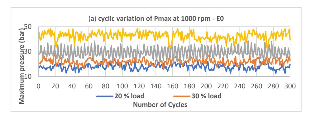
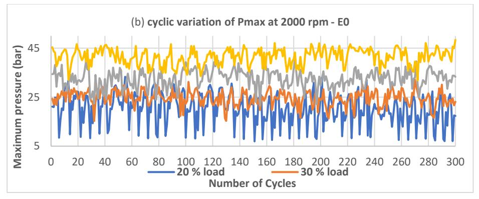
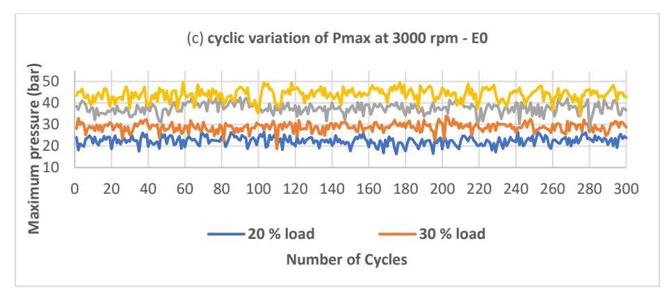
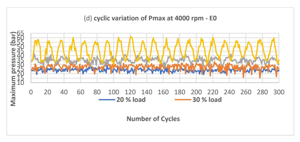
Figure 2 Cyclic variation of maximum combustion pressure.
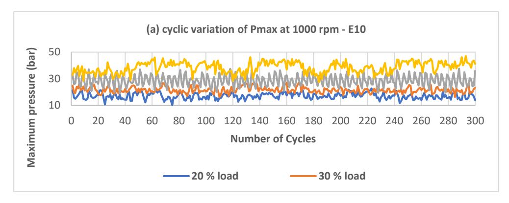
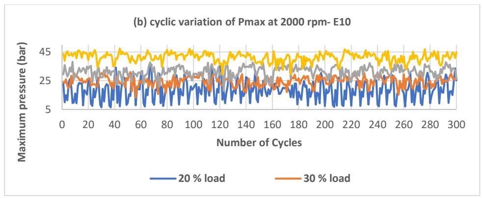
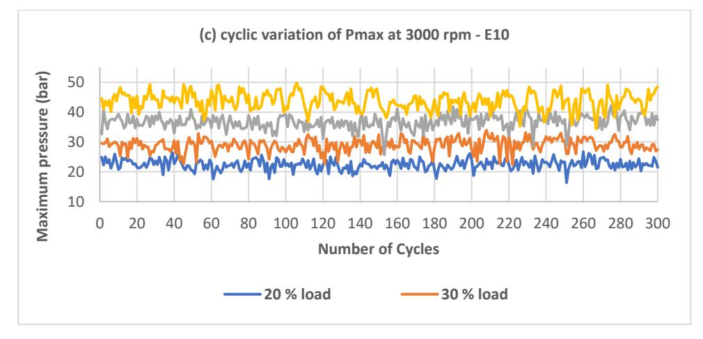
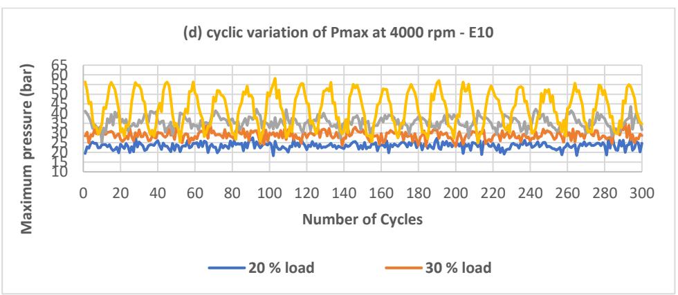
Cyclic variation of maximum combustion pressure.
The visualizations presented in Figures 2(a) to 2(d), Figures 3(a) to 3(d), and data from Table 9 offer detailed insights into the cycle-to-cycle variations of Pmax during the combustion process under varying load conditions. The least variation of around 9.982 bar was observed at 1000 rpm and 20% load for E0 fuel, whereas the least variation of 10.435 bar was observed at 3000 rpm and 20% load point for E10 fuel. On the other hand, it is evident from the data that the highest magnitude of Pmax fluctuations occurs at 4000 rpm and 50% load for both fuels analyzed in this study. The maximum variation for Pmax was 31.615 bar and 33.433 bar, respectively, for E0 and E10 fuel at 4000 rpm and 50% load. This finding underscore that, at 4000 rpm and a medium load condition, the engine exhibits significant instability in peak pressure (Pmax), indicating pronounced cycle-to-cycle variability. Such variations contribute to reduced combustion efficiency, potential mechanical stress, and increased wear over prolonged operation, adversely affecting long-term engine performance. This conclusion of the worst operating point of the engine is derived based on the single combustion parameter, which is peak combustion pressure (Pmax) only. So, it became essential to use the other technique, which can utilize multiple parameters together to provide a comprehensive result. Hence, to achieve a more complete understanding of engine performance and stability, further analysis was conducted using the Grey Relational Analysis (GRA) methodology. This technique utilizes multiple combustion metrics, providing a more complete evaluation of engine behavior.
Table 9 Comparison of Pmax variations for different speeds and loads for E0 and E10.
| Speed (rpm) | Load (%) | Pmax - bar (E0) | Pmax - bar (E10) | ||||
|---|---|---|---|---|---|---|---|
| Minimum | Maximum | Variation | Minimum | Maximum | Variation | ||
| 1000 | 20 | 12.464 | 22.446 | 9.982 | 10.298 | 22.807 | 12.509 |
| 1000 | 30 | 15.546 | 28.34 | 12.794 | 16.283 | 29.999 | 13.716 |
| 1000 | 40 | 20.67 | 38.551 | 17.881 | 19.176 | 37.643 | 18.467 |
| 1000 | 50 | 32.064 | 48.488 | 16.424 | 27.452 | 47.153 | 19.701 |
| 2000 | 20 | 6.954 | 33.314 | 26.360 | 6.439 | 36.786 | 30.347 |
| 2000 | 30 | 15.245 | 32.147 | 16.902 | 13.187 | 32.283 | 19.096 |
| 2000 | 40 | 21.568 | 40.154 | 18.586 | 17.979 | 38.202 | 20.223 |
| 2000 | 50 | 31.893 | 48.359 | 16.466 | 29.42 | 47.488 | 18.068 |
| 3000 | 20 | 16.244 | 26.596 | 10.352 | 16.332 | 26.767 | 10.435 |
| 3000 | 30 | 18.676 | 33.978 | 15.302 | 22.325 | 33.932 | 11.607 |
| 3000 | 40 | 28.211 | 43.227 | 15.016 | 25.67 | 42.746 | 17.076 |
| 3000 | 50 | 34.458 | 49.691 | 15.233 | 34.395 | 49.798 | 15.403 |
| 4000 | 20 | 19.017 | 29.582 | 10.565 | 18.295 | 29.248 | 10.953 |
| 4000 | 30 | 15.174 | 33.402 | 18.228 | 23.043 | 35.482 | 12.439 |
| 4000 | 40 | 27.276 | 42.382 | 15.106 | 25.155 | 43.709 | 18.554 |
| 4000 | 50 | 29.66 | 61.275 | 31.615 | 24.786 | 58.219 | 33.433 |
Grey Relational Analysis (GRA) Optimization Method
Grey Relational Analysis (GRA) is a multi-criteria optimization method based on the grey system theory. This theory utilizes information and its interrelationships in a "grey" context. The GRA method is widely used in industry to tackle various problems related to manufacturing, process, service, design of experiments, and many more (Zhang et al., 2023).
Grey Relational Analysis (GRA) finds the upper hand when compared to other optimization techniques, as GRA can effectively function with a limited dataset compared to the extensive and complete dataset requirement of other methods. Hence, the GRA technique became beneficial in scenarios where very limited or partial data is available from the experiments. Due to the limited data available in the present study, GRA became the ideal choice among the other optimization techniques. Moreover, GRA can tackle multiple interrelated indicators such as maximum pressure (Pmax), pressure fluctuations, combustion duration, and emissions very efficiently. GRA provides a ranking of different operating conditions by generating a relational grade that quantifies how closely each condition aligns with an ideal reference (Sathish Kumar et al., 2023). As a result, GRA proves to be exceptionally valuable for comparing engine performance
across various RPM and load conditions for this study, enabling the identification of scenarios that present the most significant challenges to stability and efficiency.
The following are the steps that make up the GRA technique.
Step 1: The first step involves the consideration of the response attributes.
Step 2: Normalizing the attributes using the quality characteristics.
The process fundamentally involves two ways of complex computation which are given as:
a) The larger the better characteristic, this is given by:
\[X_i = \frac{x_i - x_{min}}{x_{max} - x_{min}}\]
b) The smaller the better characteristic, this is given by:
\[X_i = \frac{x_{max} - x_i}{x_{max} - x_{min}}\] where, \(X_i\) is the normalized value of the attribute, \(x_i\) is the \(i^{th}\) value of the attribute, \(x_{max}\) is the maximum value of the attribute and \(x_{min}\) is the minimum value of the attribute.
Step 3: Calculating the deviation sequence which is given as:
\[a_i = 1 - X_i\]
Step 4: Calculating the Grey Relational Coefficient which is given as:
\[A_i = \frac{a_{min} + 0.5 * a_{max}}{a_i + 0.5 * a_{max}}\]
Step 5: Calculating the Grey Relational Grade (GRG) which is given as:
\[GRG = \frac{1}{n} \sum_{j=1}^{n} A_{ij}\]
Step 6: Ranking based on grey relational grade to find the best alternatives
Table 10 The Rank based best alternative using GRA the experimental runs on E0 fuel.
| Speed (RPM) | Load (%) | DS_Pmax | DS_IMEP_COV | DS_MBF50 | DS_Brn_drn | GRG | Rank |
|---|---|---|---|---|---|---|---|
| 1000 | 20 | 0.333 | 0.927 | 0.371 | 0.371 | 0.501 | 13 |
| 1000 | 30 | 0.370 | 0.962 | 0.333 | 0.333 | 0.500 | 14 |
| 1000 | 40 | 0.459 | 0.566 | 0.385 | 0.501 | 0.478 | 15 |
| 1000 | 50 | 0.819 | 1.000 | 0.554 | 0.552 | 0.731 | 4 |
| 2000 | 20 | 0.354 | 0.337 | 0.348 | 0.603 | 0.411 | 16 |
| 2000 | 30 | 0.398 | 0.908 | 0.463 | 0.676 | 0.611 | 11 |
| 2000 | 40 | 0.515 | 0.899 | 0.546 | 0.672 | 0.658 | 6 |
| 2000 | 50 | 0.765 | 1.000 | 0.694 | 0.762 | 0.805 | 2 |
| 3000 | 20 | 0.374 | 0.333 | 0.633 | 0.667 | 0.502 | 12 |
| 3000 | 30 | 0.452 | 0.530 | 0.724 | 0.846 | 0.638 | 7 |
| 3000 | 40 | 0.631 | 0.491 | 0.983 | 0.763 | 0.717 | 5 |
| 3000 | 50 | 0.883 | 0.651 | 1.000 | 0.916 | 0.862 | 1 |
| 4000 | 20 | 0.389 | 0.653 | 0.622 | 0.887 | 0.638 | 8 |
| 4000 | 30 | 0.433 | 0.670 | 0.473 | 0.888 | 0.616 | 10 |
| 4000 | 40 | 0.563 | 0.551 | 0.526 | 0.861 | 0.625 | 9 |
| 4000 | 50 | 1.000 | 0.455 | 0.761 | 1.000 | 0.804 | 3 |
| Speed (RPM) | Load (%) | DS_Pmax | DS_IMEP_COV | DS_MBF50 | DS_Brn_drn | GRG | Rank |
|---|---|---|---|---|---|---|---|
| 1000 | 20 | 0.333 | 0.925 | 0.439 | 0.341 | 0.509 | 14 |
| 1000 | 30 | 0.376 | 0.993 | 0.441 | 0.333 | 0.536 | 13 |
| 1000 | 40 | 0.470 | 0.597 | 0.465 | 0.366 | 0.475 | 15 |
| 1000 | 50 | 0.721 | 1.000 | 0.591 | 0.396 | 0.677 | 7 |
| 2000 | 20 | 0.347 | 0.333 | 0.333 | 0.494 | 0.377 | 16 |
| 2000 | 30 | 0.410 | 0.930 | 0.582 | 0.557 | 0.620 | 12 |
| 2000 | 40 | 0.519 | 0.986 | 0.624 | 0.578 | 0.677 | 8 |
| 2000 | 50 | 0.846 | 0.996 | 0.809 | 0.645 | 0.824 | 2 |
| 3000 | 20 | 0.385 | 0.541 | 0.768 | 0.884 | 0.645 | 10 |
| 3000 | 30 | 0.475 | 0.642 | 0.825 | 0.872 | 0.703 | 6 |
| 3000 | 40 | 0.656 | 0.573 | 0.931 | 0.883 | 0.761 | 4 |
| 3000 | 50 | 1.000 | 0.582 | 1.000 | 0.883 | 0.866 | 1 |
| 4000 | 20 | 0.396 | 0.466 | 0.676 | 0.957 | 0.624 | 11 |
| 4000 | 30 | 0.474 | 0.537 | 0.639 | 1.000 | 0.662 | 9 |
| 4000 | 40 | 0.624 | 0.613 | 0.678 | 0.991 | 0.726 | 5 |
| 4000 | 50 | 0.909 | 0.476 | 0.690 | 0.998 | 0.768 | 3 |
Table 11 The Rank based best alternative using GRA the experimental runs on E10 fuel.
The GRA procedure was executed in Microsoft Excel as per the aforementioned steps using larger the better characteristic for Pmax and smaller the better characteristic for the remaining combustion parameters.
Tables 10 and 11, respectively, display the ranking hierarchies for the experimental runs of the E0 and E10 fueled engines. In Tables 10 and 11, the deviation sequences (DS) represent the normalized deviation of specific performance attributes, while the grey relational grade (GRG) signifies the comprehensive performance metric obtained through the Grey Relational Analysis (GRA) multi-criteria optimization approach. Utilizing this method on the analyzed mean engine combustion data, it was determined that the operating condition of 3000 rpm at a 50% load yielded the highest GRG score of 0.866. This outcome indicates that the aforementioned condition achieved optimal engine performance and was subsequently ranked as the top-performing scenario among all tested engine operating conditions for both pure gasoline (E0) and ethanol-blended fuel (E10).
Conversely, the analysis revealed that the operating condition of 2000 rpm at a 20% load demonstrated the lowest GRG score, marking it as the least efficient alternative in the context of engine combustion performance as evaluated by the GRA method. These findings provide a foundation for subsequent research and optimization strategies in the field of internal combustion engines. Future investigations could specifically concentrate on re-calibrating and optimizing engines that use blended fuels. The aim would be to improve combustion characteristics, even under suboptimal conditions, such as those observed at 2000 rpm and 20% load. By fine-tuning the calibration, researchers can potentially address performance deficiencies and achieve more consistent and efficient combustion across different engine operating conditions.
Forecasting of Combustion parameters using Machine Learning
Machine learning-based forecasting results of two important combustion parameters, viz., start of combustion (SOC) and Pmax are presented in this section. In this study, machine learning models were developed, which are capable of predicting peak combustion pressure (Pmax) and start of combustion (SOC) in an engine based on engine speed and load conditions. The methodology and experimental process were designed to ensure that the model is reliable, accurate, and robust ultimately eliminating the need for actual testing.
Trials and Data Acquisition: In this study, 32 distinct runs were performed on the engine. That means engine data was captured for 32 different engine speeds and load points. For each unique point, in-cylinder data for 300 combustion cycles were recorded with the help of the HSDA system. This results in a total of 9600 data points collected for 32 test points (9600 data points = 300 cycles X 32 test runs). These data points capture the engine's performance characteristics, including in-cylinder combustion parameters like peak combustion pressure, start of combustion (SOC), burn duration, etc., during each cycle.
Cycle-to-Cycle Variations: In actual engine operation, each combustion cycle can vary differently from the next, even under seemingly identical conditions. These variations can be caused by factors such as temperature fluctuations, fuel
variations, mechanical wear, etc. The machine learning model had to address the inherent variation that occurs from cycle to cycle. This was crucial for the model to consistently predict the start of combustion (SOC) and maximum power output (Pmax) despite the fluctuations between cycles. Additionally, the study emphasized the importance of using comprehensive and realistic data to train the machine learning model. This approach enabled the model to learn from data that closely reflects the dynamic and sometimes unpredictable nature of real engine operation, rather than relying only on idealized or controlled conditions.
Application of Machine Learning (Random Forest)
Due to its accurate predictions and computational efficiency across different types of classification and regression applications, the random forest method has been widely used for a variety of machine-learning problems (Elumalai et al., 2022; Khoshkangini et al., 2023; Sebayang et al., 2017; Shin et al., 2020; Sonawane et al., 2023; Yang et al., 2022). This algorithm comprises an ensemble of decision trees, each tailored to user-defined metrics, which collectively contribute to generating the final decision values. The workflow of this algorithm is depicted in Figure 4. The scikit-learn library resource in python was utilized to apply random forest algorithm on the combustion data collected in the present study. The experimental data was split into 80:20 ratio for training and testing respectively.
As mentioned before, maximum combustion pressure and SOC were predicted using the random forest model. The R squared (\(R^2\)) and mean squared error (MSE) metrics were selected to verify the accuracy of model predictions. The MSE and \(R^2\) are expressed as follows:
\[MSE = \frac{1}{n} \sum_{i=1}^{n} (P_i - A_i)^2\] (6)
\[R^2 = 1 - \frac{\sum_{i=1}^{n} (P_i - A_i)^2}{\sum_{i=1}^{n} (A_i - \mu)^2}\] (7)
Where, \(P_i\) is the predicted value of \(i^{th}\) observation, \(A_i\) is the actual value of \(i^{th}\) observation, \(\mu\) is the mean value of the actual observations and N is the number of observations
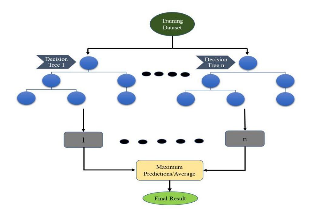
Figure 4 Flow chart of Random Forest Method.
The MSE and \(R^2\) prediction accuracies for Pmax and SOC are shown in Table 12. These results indicate excellent prediction accuracy (in terms of \(R^2\) 90% and above) of the random forest-based machine learning model developed in the current study. The MSE values are also quite low (less than 5%) for both combustion parameters.
| Table 12 R | 2 and MSE score of combustion characteristics on experimental data. |
|---|
| Attributes | 2 R score | MSE |
|---|---|---|
| Pmax | 0.91 | 2.97 |
| SOC | 0.90 | 3.03 |
Specifically, the prediction accuracy for peak pressure in combustion cycles shows a promising result with R 2 being greater than 0.9 and MSE being less than 3. The machine learning procedure adopted in the present study also ensures a reliable prediction accuracy for SOC, which is a complex parameter that changes from cycle to cycle during combustion. The cycle to cycle variations are primarily caused due to deviations in the fuel mixture compositions as well as thermal distribution differences (Duan et al., 2021). These factors lead to partial combustion or even misfiring in the engine cylinder, which makes these parameters difficult to predict. Accurate predictions of these combustion parameters are important for precise engine calibrations to achieve better fuel efficiency and minimize emissions. The predicted vs. tested Pmax and SOC results were plotted on box plots for proper visualization of their mutual variability. The machine learning prediction versus actual engine data box plots shown in Figure 5 clearly depict negatively skewed data for the start of combustion in the combustion chamber. Figure 6 also shows a slightly left skewed data for the predicted and actual Pmax. These box plot distributions will help engineers to effectively calibrate operating parameters for optimum performance of E0 and E10 fueled engines. Figure 5 shows SOC averaging at -5˚ in both predicted and actual plots. These plots also show a few outliers in the range of 5˚ to 45˚. This result is an important finding for engine calibration engineers to consider retarding or advancing the combustion cycle for achieving the corresponding performance and emission characteristics while using E0 and E10 fuels. This prediction of outliers in this regard is also important as these outliers indicate misfiring on cycle to cycle basis. Figure 6 shows Pmax averaging at 29 bars. There are no outliers in this case. These plots provide key insights into the deeper mechanisms of fuel burning/combustion instabilities in the engine. Therefore, machine learning could play a vital role in a better understanding of the fuel burning dynamics of E0/E10 fueled engines.
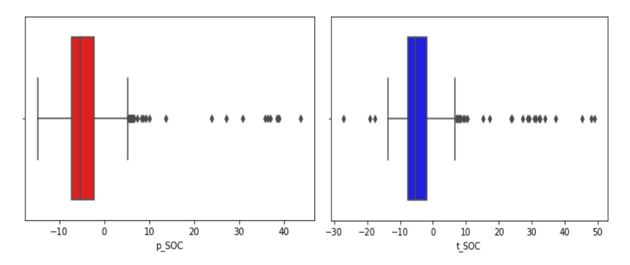
Box plot representations of prediction (in red) vs actual (in blue) for start of combustion
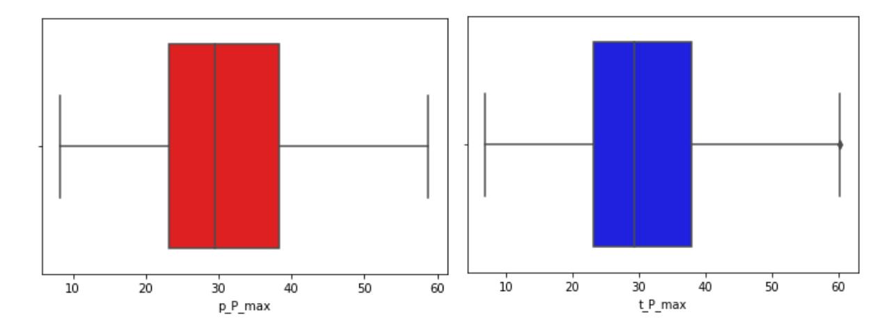
Box plot representations of prediction (in red) vs actual (in blue) for maximum pressure in each cycle.
The developed machine-learning models were subsequently evaluated for their predictive accuracy under intermediate speed and load conditions, which were not included in the original training dataset. This testing phase aimed to assess the model's ability to generalize beyond the data it was trained on, providing insights into its real-world applicability.
Table 13 compares the tested and predicted values of peak pressure (Pmax) for two fuel types, E0 and E10 at intermediate speed and load conditions. The percentage deviation between the tested and predicted Pmax values ranged from -7.93% to 9.85% for E0 and -8.08% to 9.33% for E10. The machine learning model demonstrated satisfactory predictive accuracy for both E0 and E10 fuels under intermediate speed and load conditions for Pmax.
| Pmax - bar (E0) | Pmax - bar (E10) | |||||||
|---|---|---|---|---|---|---|---|---|
| Speed (rpm) | Load (%) | Tested | Predicted | Variation (%) | Tested | Predicted | Variation (%) | |
| 1500 | 20 | 19.12 | 17.54 | 8.26 | 18.98 | 17.21 | 9.33 | |
| 1500 | 30 | 23.35 | 21.65 | 7.28 | 23.25 | 21.4 | 7.96 | |
| 1500 | 40 | 27.89 | 25.53 | 8.46 | 26.89 | 24.89 | 7.44 | |
| 1500 | 50 | 42.11 | 41.62 | 1.16 | 40.02 | 38.37 | 4.12 | |
| 2500 | 20 | 21.21 | 19.12 | 9.85 | 20.86 | 19.25 | 7.72 | |
| 2500 | 30 | 26.82 | 28.62 | -6.71 | 26.98 | 28.61 | -6.04 | |
| 2500 | 40 | 35.21 | 36.77 | -4.43 | 34.15 | 36.09 | -5.68 | |
| 2500 | 50 | 42.75 | 41.66 | 2.55 | 42.81 | 41.42 | 3.25 | |
| 3500 | 20 | 23.19 | 23.75 | -2.41 | 23.05 | 23.78 | -3.17 | |
| 3500 | 30 | 28.33 | 28.31 | 0.07 | 29.08 | 30.15 | -3.68 | |
| 3500 | 40 | 36.38 | 38.13 | -4.81 | 36.45 | 37.91 | -4.01 | |
| 3500 | 50 | 49.95 | 53.91 | -7.93 | 48.89 | 52.84 | -8.08 | |
Table 13 Comparison of predicted and tested Pmax
Table 14 compares the tested and predicted values of the start of combustion (SOC) for two fuel types, E0 and E10. The percentage deviation between the tested and predicted SOC values ranges from -9.11% to 11.11% for E0 and -7.96% to 10.53% for E10. Hence, the machine learning model demonstrated satisfactory predictive accuracy for both E0 and E10 fuels under intermediate speed and load conditions for SOC as well.
Following the machine learning methodology adopted in the present study, several more blend sets can also be anticipated and verified in accordance with the specifications of calibration experts. This methodology could also help to better understand the impact of cyclic variations on the engine under several loading conditions. The GRA methodology is also very useful to optimize engine operation. Once the ranking of the experimental parameters is tabulated, it becomes very easy to identify the highest and lowest-ranked experimental runs. These results can be taken forward to resolve the engine operation zone bottlenecks. Detailed and focused analysis of these bottlenecks will reveal deeper aspects of fuel-burning dynamics under varying loading conditions.
| SOC – Deg BTDC (E0) | SOC – Deg BTDC (E10) | ||||||
|---|---|---|---|---|---|---|---|
| Speed (rpm) | Load (%) | Tested | Predicted | Variation (%) | Tested | Predicted | Variation (%) |
| 1500 | 20 | -0.54 | -0.48 | 11.11 | 0.7 | 0.73 | -4.29 |
| 1500 | 30 | -0.85 | -0.77 | 9.41 | 1.05 | 1.12 | -6.67 |
| 1500 | 40 | -1.45 | -1.49 | -2.76 | 0.95 | 0.85 | 10.53 |
| 1500 | 50 | -2.25 | -2.1 | 6.67 | -0.78 | -0.7 | 10.26 |
| 2500 | 20 | -7.1 | -6.4 | 9.86 | -5.4 | -5.83 | -7.96 |
| 2500 | 30 | -6.3 | -6.82 | -8.25 | -5.95 | -6.27 | -5.38 |
| 2500 | 40 | -7.9 | -8.62 | -9.11 | -6.8 | -7.3 | -7.35 |
| 2500 | 50 | -7.35 | -7.8 | -6.12 | -7.05 | -7.5 | -6.38 |
| 3500 | 20 | -7.8 | -7.23 | 7.31 | -6.75 | -7.26 | -7.56 |
| 3500 | 30 | -4.85 | -4.45 | 8.25 | -6.15 | -5.54 | 9.92 |
| 3500 | 40 | -5.58 | -5.05 | 9.50 | -5.68 | -5.33 | 6.16 |
| 3500 | 50 | -5.65 | -5.08 | 10.09 | -5.76 | -5.16 | 10.42 |
Table 14 Comparison of predicted and tested SOC
The Taguchi-GRA-Random Forest methodology presented in the current work helps calibration engineers to understand the cycle-to-cycle variation in a better manner and also potentially reduces the entire duration and expense of a new research and development project using blended fuels. The comparison of algorithms with various sets of blends can be an idealistic approach to expand this study to comprehend the impact of higher oxygenated fuels on combustion cyclic variability.
Application of Machine Learning (Artificial Neural Network)
Furthermore, the outcome of the Random Forest Machine Learning model was compared with the output from the Artificial Neural Network (ANN) model for the same dataset. The implemented Artificial Neural Network (ANN) consisted of a 2-layered feedforward network designed for predicting outcomes based on input features. The key characteristics and configurations of this ANN architecture are shown in Figure 7 and explained below.
ANN Architecture
The input layer accepts the input features that represent the relevant parameters for the problem at hand. The size of the input layer corresponds to the number of features in the dataset. In this study, the dataset that was used for Random Forest was fed to the ANN model as well. A total of 9,600 data points collected across all trials were used as input for ANN modeling. The SOC and Pmax for E0 and E10 were predicted using the ANN model. A sigmoid activation function was applied in the hidden layer to introduce non-linearity. Finally, the output layer produced the final predicted values.
Two-layered feed forward neural networks (Al-Aboodi et al., 2017).
Working Mechanism of Feed Forward Network
In this network, the input data is passed through the network, layer by layer. Weights and biases are applied to transform the inputs at each layer. The sigmoid activation function in the hidden layer allows the network to capture
non-linear patterns in the data. During training, weights and biases are adjusted iteratively using backpropagation and an optimization algorithm, such as gradient descent. This process aims to minimize the error between the predicted output and the actual output.
Algorithm Settings
The following algorithm settings were used during the ML modeling:
Data division: Random
Training algorithm: Levenberg-Marquardt.
The termination criteria defined for this network is shown in Table 15.
Table 15 Termination Criteria
| Unit | Target Value | ||
|---|---|---|---|
| Epoch | 1000 | ||
| Elapsed Time | ∞ | ||
| Performance | 0 | ||
| Gradient | 1e-07 | ||
| Mu | 1e+10 | ||
| Validation Checks | 6 | ||
Output
The performance output of the ANN model for predicting Pmax (maximum pressure) and SOC (start of combustion) for two fuel types, E0 (pure gasoline) and E10 (10% ethanol blend), is tabulated in Table 16. The performance was evaluated using the R² score (coefficient of determination) and Mean Squared Error (MSE).
Table 16 R 2 and MSE score for ANN Predictions
| Attributes | 2 R | score | MSE | |
|---|---|---|---|---|
| E0 | E10 | E0 | E10 | |
| Pmax | 0.9462 | 0.9478 | 9.8964 | 8.8539 |
| SOC | 0.6506 | 0.6521 | 16.3086 | 19.1537 |
The model establishes strong performance in predicting Pmax, as evidenced by high R² values and low mean squared error (MSE) for both fuel types. The slightly better performance for E10 suggests that the model effectively captures the combustion dynamics of ethanol-blended fuel. In contrast, the model's performance in predicting SOC is moderate, displaying lower R² values and higher MSE compared to Pmax. The marginally improved metrics for E10 indicate that the model adapts somewhat more effectively to the characteristics of ethanol-blended fuel when predicting SOC, although there is still significant room for improvement.
Comparison with Random Forest ML model
The outcome of the Random Forest (RF) model illustrates notable predictive accuracy for both Pmax (maximum pressure) and SOC (start of combustion). The R² scores of 0.91 for Pmax and 0.90 for SOC indicate high level of reliability. Furthermore, the low Mean Squared Error (MSE) values of 2.97 for Pmax and 3.03 for SOC highlight the model's effectiveness in making precise predictions with minimal error. Overall, this level of accuracy shows that the model is reliable and capable of forecasting combustion dynamics under a variety of circumstances.
Thus, the Random Forest (RF) model can overcome the accuracy constraints that often affect the use of Artificial Neural Networks (ANNs). This ensemble approach improves generalization and decreases overfitting. Unlike ANNs, which can be sensitive to noise and require extensive tuning, RF builds multiple decision trees using random subsets of both data and features. By averaging the predictions from these trees, RF improves stability and accuracy. This makes RF particularly effective for handling non-linear relationships and complex interactions, such as those influencing the start of combustion (SOC). Furthermore, RF is less dependent on big datasets and is capable of processing numerical and categorical data, which makes it appropriate for situations with little data. Its capability to rank feature importance provides valuable insights, enabling targeted data collection or refinement of input features. For SOC prediction, RF's
resilience to outliers and its ability to model subtle interactions between variables such as fuel properties, load, and speed can significantly enhance performance.
Calibration Strategies Based on GRA Results
Based on the findings of the study, 2000 rpm and 20% load conditions were found to be critical engine load and speed conditions. Following engine calibration strategies can be used to mitigate the effect of the particular engine operating point.
- 1. Ignition Timing Optimization: Calibrating the ignition timing more accurately could help to reduce cycle-to-cycle variability and enhance combustion efficiency. During the engine optimization process, the engine has to be set to 2000 rpm and 20% load by using the engine dynamometer speed-torque mode. Once the engine is set to the desired condition, the calibration engineer has to vary the ignition timing by 2-3° in the step of 0.5° to arrive at the optimal ignition timing corresponding to the least possible fluctuations in Pmax.
- 2. Air-Fuel Ratio (Lambda) Control: Improving the control systems for adjusting the air-fuel mixture can achieve optimal combustion based on predicted Start of Combustion (SOC) and Peak Pressure (Pmax) values. This may lead to better fuel economy and lower emissions by minimizing incomplete combustion. Once the engine is set to the desired condition, the calibration engineer has to vary the air-fuel ratio (λ) around 1 (λ =1, stoichiometric condition) by adjusting the throttle body opening and fuel delivery. The λ is varied from 0.995 to 1.005 to achieve the optimum engine combustion performance.
- 3. Engine Load and Speed Management: Implementing adaptive strategies for managing engine load and speed, particularly in operational regimes highlighted by the study as prone to irregular combustion. This includes realtime monitoring and adaptive calibration algorithms to address performance issues under low-load and low-speed conditions.
- 4. Knocking Detection and Mitigation: The knock detection system can be refined by utilizing predictive SOC and Pmax data. Improved calibration can proactively adjust ignition timing and fuel delivery to prevent engine knock, thereby enhancing the engine's longevity and reliability.
- 5. Engine Control Algorithms (Real-Time): Predictive data can be used simultaneously in advanced real-time control algorithms to adjust the multiple engine parameters, ensuring consistent performance across various operating conditions.
- 6. These calibration enhancements, based on the study's insights into cycle-to-cycle variations and predictive modeling, could greatly enhance engine performance, efficiency, and emissions control.
Conclusions
The cycle-to-cycle variations of in-cylinder combustion parameters in spark ignition (SI) engines operating on E0 and E10 fuel blends were examined in this study. The full factorial Taguchi method was used to define the test matrix. Accordingly, experimentation was conducted with both E0 and E10 fuels. The in-cylinder combustion data was captured using the HSDA system, and parameters like peak combustion pressure (Pmax), burn duration, and IMEP were derived. After analyzing the data, considerable cycle-to-cycle variation was observed for Pmax and other combustion parameters. Furthermore, the Grey Relational Analysis (GRA) technique was used to identify the optimal and suboptimal operating conditions for both E0 and E10 fuels. The research highlighted a gap in the existing literature, suggesting the promising application of machine learning techniques to correlate these variations with different engine operating conditions. Considering this, random forest and artificial neural network machine learning modeling were applied to the engine test data to predict the start of combustion (SOC) and maximum combustion pressure (Pmax) under various engine RPM and load scenarios. A total of 9600 data points gathered over 32 test runs was used to train and test the machine learning models. Box plots were employed for comparative visualization between actual and predicted SOC and Pmax results. The summary of the research findings is presented as follows:
- 1. The highest magnitude of Pmax fluctuations occurs at 4000 rpm and 50% load for both fuels analyzed in this study. The lowest magnitude of Pmax fluctuations occurs at 1000 rpm and 10% load for E0 and at 3000 rpm and 20% load for E10 Fuel.
- 2. Grey Relational Analysis (GRA) showed that the 3000 rpm and 50% load combination was optimal, while the 2000 rpm and 20% load conditions were the least favorable.
- 3. The Random Forest model's prediction accuracy for SOC and Pmax was confirmed by R-squared values exceeding 90% and mean squared errors below 3%.
- 4. The Random Forest machine learning model predicted an average SOC of -5° crank angle and a maximum pressure of 29 bars, thus providing reliable data for recalibration to enhance engine performance and emissions.
- 5. The ANN model predicts Pmax accurately, with better performance for E10, while SOC predictions are moderate, highlighting the need for improvement, especially for ethanol-blended fuels.
The primary outcome of this machine learning-based approach is to predict the engine operating characteristics of E0 and E10 fuel at any combination of engine rpm and loading conditions. This methodology reduces the time and cost of testing the engine under different conditions. Also, this study shows that the issues related to cyclic variations at part load engine operating conditions can be identified and managed by operating the engine at optimal speed-load conditions.
Conflict of Interest Statement
The authors declare that the research was conducted without any financial or commercial relationships that could be construed as a potential conflict of interest.