
Introduction
Java Island lies in a tectonically active region, where the Australian Plate subducts beneath the Sunda Block (Bird, 2003) in the northeast direction. The convergence rate along the Java Trench varies, with the western part experiencing a
Swiss Seismological Service (SED), ETH Zürich, Sonnegstrasse 5, Zürich 8006, Switzerland
2Geophysical Engineering Department, Faculty of Civil, Planning and Geo Engineering, Institut Teknologi Sepuluh Nopember, Jalan Raya ITS, Sukolilo, Surabaya 60111, Jawa Timur, Indonesia.
Indonesian Agency for Meteorology Climatology and Geophysics (BMKG), Jalan Angkasa I No. 2 Kemayoran, Jakarta Pusat 10610, Jakarta, Indonesia
4Global Geophysics Research Group, Faculty of Mining and Petroleum Engineering, Institut Teknologi Bandung, Jalan Ganesa No. 10 Bandung 40132, Jawa Barat, Indonesia
5Earthquake Research Group, Geological Disaster Research Center, National Research and Innovation Agency (BRIN), Jalan Sangkuriang, Dago, Bandung 40135, Jawa Barat, Indonesia
8Prodi Geofisika, Fakultas Matematika dan Ilmu Pengetahuan Alam, Universitas Indonesia, convergence rate of ~6 cm/year (Koulali et al., 2017). The seismicity rate in Java is highly influenced by the convergence of the two plates which are Indian-Australian and Eurasia plate (Widiyantoro et al., 2020), which results in a predominantly north-south compressive stress controlling the active faulting. However, analyses of earthquake slip vectors and global positioning system (GPS) measurements in the western part of Java indicate that the convergence is oblique, requiring left-lateral motion along the crustal faults, such as the Lembang Fault.
The Lembang Fault is one of the active crustal faults in the western part of Java (Daryono et al., 2019; Supendi et al., 2018) and has been suggested to have a left-lateral kinematic (Afnimar et al., 2015), as shown in Figure 1. The topography clearly depicts it as an east-west trending escarpment about 10 km north of Bandung City, the capital city of West Java province, with a population of over 2 million people. This fault is considered a continuation of the northern end of the Cimandiri-Rajamandala Fault. Historical records indicate that major local earthquakes heavily shook Bandung and nearby cities in 19,620–19,140 BP, 2300–60 BCE, 15th century (Daryono et al., 2019), 1863, 1873, 1879, and 1900 (Martin et al., 2022). Although the Lembang Fault is seismically active (Figure 1), no large destructive earthquakes have been instrumentally recorded. The most recent small magnitude of noticeable earthquakes is listed in Table 1.
Table 1 Historical earthquakes surround the Lembang Fault, as shown in Figure 1. The earthquake catalog is inferred from Agency of Meteorology, Climatology, and Geophysics (BMKG).
| Time | Longitude | Latitude () | Depth (km) | Magnitude (𝑴𝒘) | Strike/Dip/Rake () | |
|---|---|---|---|---|---|---|
| () | Plane 1 | Plane 2 | ||||
| 2013-05-29 12:39:04.333 | 107.63311 | -6.82143 | 12 | 3.8 | 289/80/51 | 186/40/164 |
| 2015-08-08 19:51:13.749 | 107.64215 | -6.84113 | 12 | 2.8 | 339/57/27 | 233/67/143 |
| 2015-08-09 02:37:51.347 | 107.76160 | -6.86198 | 14 | 2.7 | 249/68/42 | 140/51/151 |
| 2015-08-09 02:37:51.347 | 107.77115 | -6.86152 | 11 | 2.8 | 235/60/39 | 122/56/143 |
| 2017-05-14 03:51:54.712 | 107.72433 | -6.86431 | 6 | 2.5 | 231/57/47 | 233/67/143 |
| 2017-12-16 02:08:23.242 | 107.52231 | -6.82211 | 15 | 2.6 | 241/73/59 | 125/35/149 |
| 2018-06-12 05:34:40.087 | 107.66165 | -6.82241 | 9 | 2.7 | 295/57/33 | 185/62/142 |
Meilano et al. (2012) estimated the slip rate of this fault to be 6 mm/year with sinistral (left-lateral) movement. Daryono et al. (2019) studied this fault in detail and divided it into 6 sections, with slip rates ranging from 2 to 6 mm/year. Recent study by Hussain et al. (2023) estimated the slip rate for the fault is 4.7 mm/year, with a shallow portion of the fault creeping segment at 2 mm/year. The fault exhibits distinct geometrical characteristics along its 29 km length, transitioning from strike-slip to vertical faulting mechanisms. Previous studies have identified the fault as both a normal fault (e.g Daryono et al. (2019); Hidayat et al. (2008); Van-Bemmelen, (1949)) with a northern dip direction and a thrust fault with a southern dip direction (e.g., Nurhasan et al. (2024)). Despite a lack of significant recorded earthquakes, the Lembang Fault is active and poses a high seismic hazard to the surrounding region. Deformation studies estimate the fault could produce earthquakes ranging from magnitude 6.7 to 7.0, though these estimates do not account for the fault's unique geometry, which includes bends at both its eastern and western ends (Daryono et al., 2019). This geometrical complexity can over- or under-estimate the maximum magnitude.
In this study, we assessed earthquake scenarios involving transitional regime of normal and reverse faulting with strikeslip faulting of the Lembang Fault using 3D physics-based dynamic rupture simulations that incorporate the fault's geometrical complexity (i.e., fault bending and non-planar surface), 3D velocity structure, and plastic deformation. We investigated the rupture dynamics, conditions leading to self-sustained rupture, and the resulting ground-motion distribution around the Lembang Fault.
In the following sections, we first describe the components of the dynamic rupture simulations. Then, in the Results section, we analysed a set of dynamic rupture simulations to assess the conditions leading to a runaway rupture, its ground-motion distributions, and the corresponding equivalent point-source properties. Finally, we validate our groundmotion results against pre-existing ground-motion models, emphasizing that our numerical simulations are realistic and robust.
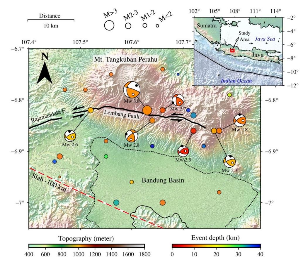
Seismicity around the Lembang Fault, with focal mechanisms for events of > 2.4 (Table 1). Black lines represent the faults (National Earthquake Study Center (PUSGEN), 2017) The earthquake catalog is inferred from the BMKG catalog. The topography data is obtained from (National Bathymetric System – Geospatial Information Agency, 2024). The Slab2.0 model is based on Hayes et al. (2018).
Model Setup
Dynamic rupture simulations are governed by initial stress conditions, fault strength, fault geometry, subsurface material properties, the nucleation procedure, and the friction law (Udias et al., 2013) (Scholz, 2018). In this study, we vary fault geometry and initial stress conditions, representing two different scenarios that may result in varying dynamics of rupture propagation and, consequently, different ground motions.
We modeled dynamic earthquake rupture scenarios using a curved plane representing the Lembang Fault. We conducted simulations for two fault plane geometries with their corresponding stress regimes. The first scenario features a fault dipping to the north at 75°, based on the fault geometry proposed by Daryono et al. (2019) (black line in Figure 1). However, the fault surface trace is simplified from the original interpretation by Daryono et al. (2019) to reduce computational complexity. The second scenario is characterized by a fault geometry dipping to the south at 75°, following the work of Nurhasan et al. (2024), who investigated this geometry using the magnetotelluric method.
Based on surface traces and geological observations, the Lembang Fault is characterized by two fault bends on either side of the fault (Figure 1). In this study, the Lembang Fault is modeled as having a length of 29 km and a width of 14 km along the dip direction (Figure 2a). Both scenarios use the same fault trace; the primary difference lies in the orientation of the fault normal (Figure 2b). The fault is confined within a numerical domain of 112 x 88 x 50 km3 cube, discretized into a mesh with varying edge lengths (Figure 2c and 2d).
3D numerical model considered in this study. (a) The 3D numerical domain. (b) Fault geometry for the two scenarios considered in this study: normal and reverse faulting. (c) Mesh for the reverse faulting scenario associated with densely populated cities, with the blue color on the fault representing the rupture front. (d) Same as (c), but for the normal faulting scenario.
We used the open-source software SeisSol (https://github.com/SeisSol/SeisSol/), which employs unstructured tetrahedral meshes to represent geometrically complex geological structures (Pelties et al., 2014; Uphoff et al., 2017). High-order basis functions of polynomial degree p = 4 were utilized, achieving fifth-order accuracy in both space and time for seismic wave propagation. The on-fault mesh has an edge length of 50 m, ensuring the capture of a minimum cohesive zone width of 100 m. The surface mesh has an edge length of 200 m, effectively capturing the topography around the Lembang Fault and its surroundings. The model comprises over 22 million tetrahedral cells, resolving frequencies up to approximately 1 Hz near the Lembang Fault. The dynamic rupture boundary condition is prescribed on the element interface (fault surface). The free surface boundary condition, which is characterized by traction free, is applied on the surface on the tetrahedral faces. We used absorbing boundary condition on the sides and bottom of the numerical mesh.
Material Properties and Initial Stress
In this study, we assumed 3D heterogeneous isotropic elasto-viscoplastic material properties to model the dynamics of the Lembang Fault scenario in half-space for both normal and reverse faulting scenarios (Figure 3). The 3D material is extracted from ambient noise tomography results in this area by Pranata et al. (2020). Their 3D S-wave velocity ( ) model was converted to P-wave velocity () using empirical scaling relation by Brocher (2005), as is valid for Vs 4.5 km/s (e.g., Lehujeur et al. (2021); Ry et al. (2023)). The 3D heterogeneous material varies up to a depth of 10 km. At deeper depth, we considered a 1D layered isotropic medium. The Lembang Fault intersects the surface topography at an elevation > 0 km.
We assumed a non-associated Drucker-Prager elasto-viscoplastic rheology. The off-fault failure criterion is based on the internal bulk cohesion and friction coefficient. We considered a constant internal friction coefficient across the entire model domain, matching the prescribed on-fault friction coefficient ( = 0.6, Table 2) (Wang et al., 2017). However, bulk cohesion was modeled as 1D depth-dependent and mimics the increased rock strength with depth. Consequently, bulk cohesion varies from 4 MPa near the surface to 5 MPa at a depth of 15 km. We set a constant mesh-independent relaxation time of 0.03 s following Wollherr et al. (2018).
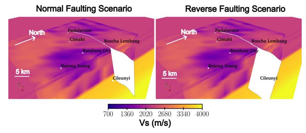
Figure 3 3D S-wave velocity (Vs) model extracted from the ambient noise tomography results by Pranata et al. (2020) for both normal and reverse faulting scenarios. The white planes indicate the Lembang Fault. Darker colors represent lower Vs values, while brighter colors depict higher Vs values.
We used a Cartesian initial stress tensor to load the fault from the ambient stress. The stress regime was constrained by the relative stress magnitude, following Simpson (1997), and is given as:
\[A_{\phi} = (n+0.5) + (-1)^{n}(\phi - 0.5) \tag{1}\] where n represents the style of faulting (n = 0 for normal faulting; n = 1 for strike-slip; and n = 2 for reverse faulting) and denotes the stress shape ratio \(\phi = \frac{(\sigma_2 - \sigma_3)}{(\sigma_1 - \sigma_3)}\). Here, \(\sigma_1\), \(\sigma_2\), and \(\sigma_3\) are the maximum, intermediate, and minimum principal stresses, respectively. The orientation of the maximum horizontal stress (\(S_{Hmax}\)) was derived from the global stress map (Heidbach et al., 2018) and verified by stress inversion from focal mechanisms around the Lembang Fault. \(S_{Hmax}\) around the Lembang Fault is approximately 50°. For the normal faulting scenario, we considered \(A_{\phi}\) = 1.2, while for the reverse faulting scenario, we used \(A_{\phi}\) = 1.9 (Table 2). The off-fault stresses were initialized consistently similar to the stresses acting on the fault. The value of \(A_{\phi}\)=1.2 can be considered indicative of a transitional regime from normal to strike-slip faulting, whereas \(A_{\phi}\)=1.9 represents a transitional regime from reverse to strike-slip faulting. These transitional regimes are taken into account due to the complexity of the Lembang Fault, which varies along its eastern, central, and western segments. However, for simplicity, we assumed a homogeneous regional ambient stress acting on the fault.
Table 2 Dynamic rupture parameter for the two scenarios.
| Parameters | Values | |
|---|---|---|
| Static Friction Coefficient (\(\mu_s\)) | 0.55 | |
| Dynamic Friction Coefficient (\(\mu_d\)) | 0.2 | |
| SHMAX | 50° | |
| Dc | 0.1 m | |
| Initial Relative Prestress Ratio (R0) | 0.6 - 0.9 | |
| R0 (Preferred) | 0.9 | |
| Fluid Pressure Ratio (\(\gamma\)) | 0.37 - 0.7 | |
| \(\gamma\) (Preferred) | 0.7 | |
| Bulk Friction Coefficient | 0.6 | |
| Nucleation Depth | 6 km | |
| Nucleation Size | 0.5 km | |
| Rigidity (\(\mu\)) | 32GPa | |
| Lamé Parameter (\(\lambda\)) | 32GPa | |
| \(A_{\boldsymbol{\phi}}\) For Normal to Strike-Slip Regime | 1.2 | |
| \(A_{\bm{\phi}}\) For Reverse to Strike-Slip Regime | 1.9 | |
Our dynamic models are characterized by linear slip weakening constitutive law, which defines linearly decreasing breakdown work during dynamic slip. The parameters consist of static (\(\mu_s\)), dynamic friction coefficients (\(\mu_d\)), and characteristics slip distance (\(D_c\)). Dynamic rupture occurs when shear stress (\(\tau\)) yields the fault strength \(\tau_s = \mu_s \sigma_n\), where \(\sigma_n\) denotes the effective confining stress that increases linearly with depth. We assumed \(\mu_s\) = 0.55, \(\mu_d\) = 0.2, \(D_c\) = 0.1 m (Table 2). The assumed of these friction coefficients are consistent with laboratory-based values of large heterogeneous lithologies (Byerlee, 1978;Di Toro et al., 2011). The Dc value is constrained by typical average slip which is related to the minimum fracture energy to propagate a rupture in moderate size earthquakes (Cocco et al., 2023).
Earthquake rupture dynamics are controlled by the relative prestress ratio R that describes the ratio of fault stress drop to breakdown strength drop, given as \(R=\frac{(\tau-\mu_d\sigma_n)}{(\mu_s-\mu_d)\sigma_n}\). \(R_0\) is the maximum possible value of R for the most optimal orientation on fault patches. Thus, R is smaller or equal to \(R_0\). It is challenging to constrain the best values for \(R_0\) to produce mechanically viable dynamic rupture, thus, we varied \(R_0\) values ranging from 0.6 to 0.9 and fluid pressure ratio (\(\gamma\), defined as the ratio of fluid pressure to background lithostatic stress) using static Coulomb stress analysis. Exploring \(R_0\) is beneficial to avoid expensive dynamic rupture simulations (Palgunadi et al., 2020, 2024).
To start the rupture, we artificially created a patch of rupture nucleation area that is prescribed in space and time by locally gradually reducing \(\mu_s\). The rupture was initiated at the hypocenter at latitude -6.82° and longitude 107.59°, and depth of 6 km. Following the setting from SCEC TPV24, the kinematic rupture initiation time T is given by:
\[T = \begin{cases} \frac{r}{0.7V_r} + \frac{0.081r_{crit}}{0.7V_r} \left( \frac{1}{1 - \left(\frac{r}{r_{crit}}\right)^2} - 1 \right), \ r \le r_{crit} \\ 10^9, \ r > r_{crit} \end{cases}\] (2)
in which r (km) is the radial distance from the hypocenter, \(r_{crit}\) = 0.5 km denotes the nucleation radius, and \(V_r\) = 3.4 km/s is the initial rupture velocity.
Results
Static and Dynamic Analysis of Initial Fault Strength
The dynamics of earthquake rupture are significantly influenced by the initial conditions which highlight the importance of providing the most detailed fault geometry, Earth's structure and stress conditions. Therefore, we conducted 40 dynamic rupture simulations and manually inspected the outcomes based on the combinations of two parameters, \(R_0\) and \(\gamma\). All other dynamic and constitutive parameters were kept constant. From these 40 simulations, the combination of \(R_0=0.9\) and \(\gamma=0.7\) produced a realistic and mechanically viable dynamic rupture. For high \(R_0\) values greater than 0.9, the scenarios were unrealistic as they resulted in rupture speeds \((V_r)\) exceeding \(V_p\). For \(R_0<0.9\) and \(\gamma<0.7\), the ruptures were considered prematurely self-arrested. Therefore, we selected \(R_0=0.9\) and \(\gamma=0.7\) for the two scenarios. These values result in a ratio of shear- to normal stress between 0.1 – 0.5, which indicates a subcritically stressed condition.
Rupture Dynamics
For the normal faulting scenario (NFS), the rupture initiates at the hypocenter and propagates bilaterally to the east and west. At t=3.4 s, the rupture fronts reach geometric discontinuities (bends) along the Lembang Fault. On the western side (indicated by the red arrow on the top left of Figure 4), there is an initiation of a rupture ahead of the primary rupture front. This feature is commonly referred to as a daughter crack (Lu et al., 2007), which could potentially lead to a supershear rupture where the rupture speed exceeds \(V_s\). On the eastern side of the Lembang Fault, the rupture front encounters the interface between lower (1.5 km/s) and higher (2.3 km/s) velocity zones, resulting in asymmetrical rupture front propagation (green arrow in the top left of Figure 4). By t=5.0 s, the rupture progresses, showing subshear rupture to the west (red arrow in the middle left of Figure 4). A smaller rupture front develops near the low and high-velocity interface (blue arrow in the middle left of Figure 4). The rupture reaches the surface at t=5.8 s on the western side of the Lembang Fault. At t=6.8 s, limited supershear rupture occurs near the surface on the west side (blue arrow in the lower left of Figure 4). The rupture front eventually ceases at the fault boundaries, dissipating in the ductile region at the deepest part of the fault. This mechanically viable dynamic rupture scenario yields a stress drop of 12.8 MPa.
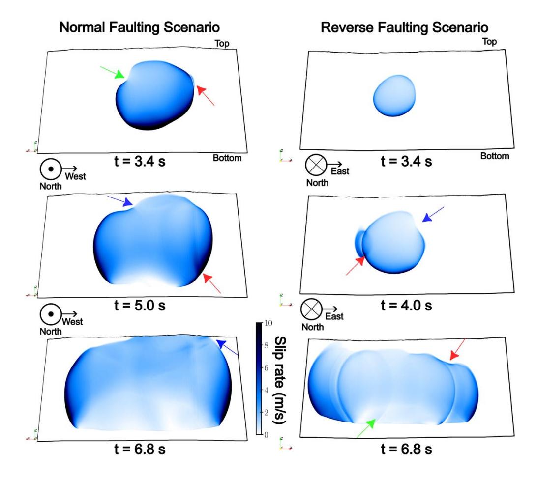
Highlights of the interesting features of the slip rate evolution for two scenarios directed toward the normal of the fault plane. The left panel shows the normal faulting scenario from t = 3.4 s to 6.8 s, while the right panel displays the reverse faulting scenario over the same time interval. The slip rate is saturated at 10 m/s.
For the reverse faulting scenario, the rupture starts more slowly than in the NFS, as indicated by the smaller slipping area at t = 3.4 s (top right panel in Figure 4), despite having the same nucleation time. At t = 4.0 s, a daughter crack forms ahead of the primary rupture front at the bend in the western part of the fault (red arrow in the middle right panel of Figure 4), similar to the NFS at t = 3.4 s. However, due to lower shear stress compared to the NFS and, therefore, weaker loading conditions, it generates a supershear rupture at about 1.5 bilaterally (as seen at t = 6.8 s, bottom right panel in Figure 4). Similar to the NFS, the rupture front at the intersection of high and low-velocity zones reduces the amplitude of the slip rate (blue arrow in the middle right panel of Figure 4). Interestingly, at the fault bend, a reflected slip rate propagates eastward (green arrow in the bottom right of Figure 4), which does not correspond to the stopping phase typically associated with the fault edge (Savage, 1965). Finally, the supershear rupture speed does not reach the surface, which might explain the lack of a clear supershear rupture signature in the surface deformation (e.g., directivity, will be explain in the following section). This scenario produces a stress drop of 5.3 MPa, twice as small as NFS.
Point Source Representation
We examined the far-field focal mechanism by calculating an equivalent moment tensor solution for a point source representation based on the corresponding slip distribution (Palgunadi et al., 2024). The fault area is considered slipping if the accumulative slip has a minimum slip of 0.01 m. In the normal faulting scenario, the slip distribution is primarily concentrated around the hypocenter (Figure 5a), extending up to the fault bend on the eastern side. The average slip for this scenario is 9.7 m. The equivalent moment tensor solution reveals a dominant double-couple strike-slip faulting mechanism (top right inset of Figure 5a, Table 3). This moment tensor solution is relatively consistent with the focal mechanisms of previous small events in this area. The resulting strike-slip focal mechanisms despite considering normalto strike-slip stress regime is because the ambient stress conditions and direction of the SHmax resulting in higher strike direction shear stress magnitude (average of 65MPa) than the dip direction (average of 20MPa).
In contrast, for the reverse faulting scenario, the slip distribution is more qualitatively spread across the fault area, with limited slip (< 1 m) on the eastern side of the fault. Surface slip for the reverse faulting scenario is limited (< 2 m) compared to the normal faulting scenario (~12 m). A slip deficit is also observed, indicated by zero slip on the surface near the fault bend on the western side of the Lembang Fault. The average slip is approximately 4.17 m. The equivalent moment tensor for the reverse faulting scenario shows a slightly non-double-couple mechanism with a positive rake, indicating a reverse faulting moment tensor solution (Table 3), with approximately -12% comprising a compensated linear vector dipole (CLVD) component. The presence of the CLVD component suggests rupture complexity due to the fault's geometric configuration (Julian et al., 1998; Palgunadi et al., 2020).
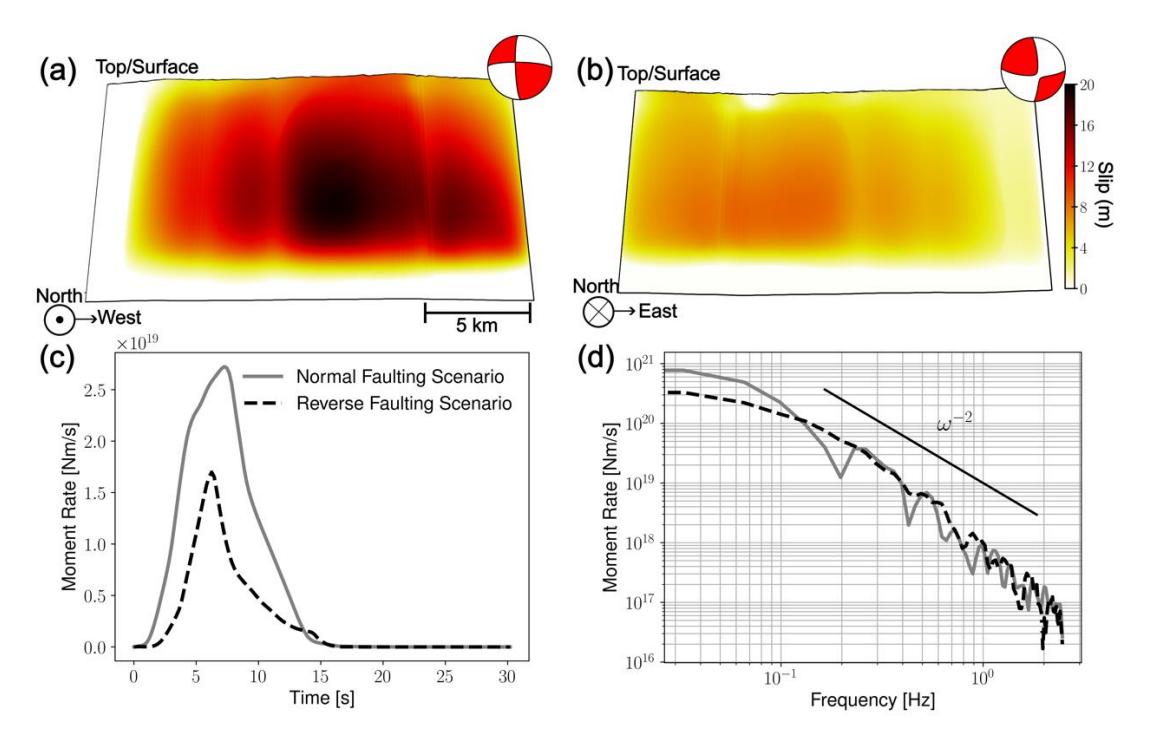
Point source representation of the two scenarios. (a) Slip distribution across the normal fault, associated with a predominantly strike-slip moment tensor solution shown at the top right. (b) Same as (a), but for reverse faulting focal mechanisms, with a low percentage (-12%) CLVD non-double-couple component. (c) Moment rate function for the two scenarios, with rupture durations of 15 s and 17 s for the normal and reverse faulting scenarios shown by grey line and black dashed line, respectively. (d) Moment rate spectra for the two scenarios, both of which follow an −2 ( = 2) Brune's model decay.
The seismic moment release for the normal and reverse faulting scenarios is 1.68 x 10²⁰ Nm ( 7.4) and 6.94 x 10¹⁹ Nm ( 7.1), respectively. Although both scenarios release seismic moments at different rates (Figure 5c), they exhibit comparable rupture durations of 16 seconds. Consequently, the overall average rupture speed is 0.8 for the normal faulting scenario and 0.9 for the reverse faulting scenario. The normal faulting scenario generates a higher seismic moment at lower frequencies (Figure 5d), indicating that the radiated seismic energy is dominated by large-scale slip across the fault plane. The reverse faulting scenario has a larger corner frequency (cut-off frequency) by approximately 0.06 Hz, which is expected due to the lower seismic moment release and, therefore, lower moment magnitude. Both moment rate releases decay following a Brune's model −2 pattern, where = 2, denotes frequency.
Table 3 Moment tensor solution from the two scenarios.
| Scenario | Strike 1 (°) | Dip 1 (°) | Rake 1 (°) | Strike 2 (°) | Dip 2 (°) | Rake 2 (°) |
|---|---|---|---|---|---|---|
| Normal Faulting | 271 | 78 | 16 | 178 | 75 | 167 |
| Reverse Faulting | 92 | 77 | 18 | 358 | 73 | 166 |
Ground Shaking Map
Our models do not account for the 3D 30 (S-wave speed for the first 30 m of depth) to reduce computational costs. As a result, the resulting shakemaps are primarily influenced by 3D dynamic ruptures, incorporating 3D values derived from tomography studies up to a depth of 0.5 km, surface topography, and off-fault plastic deformation.
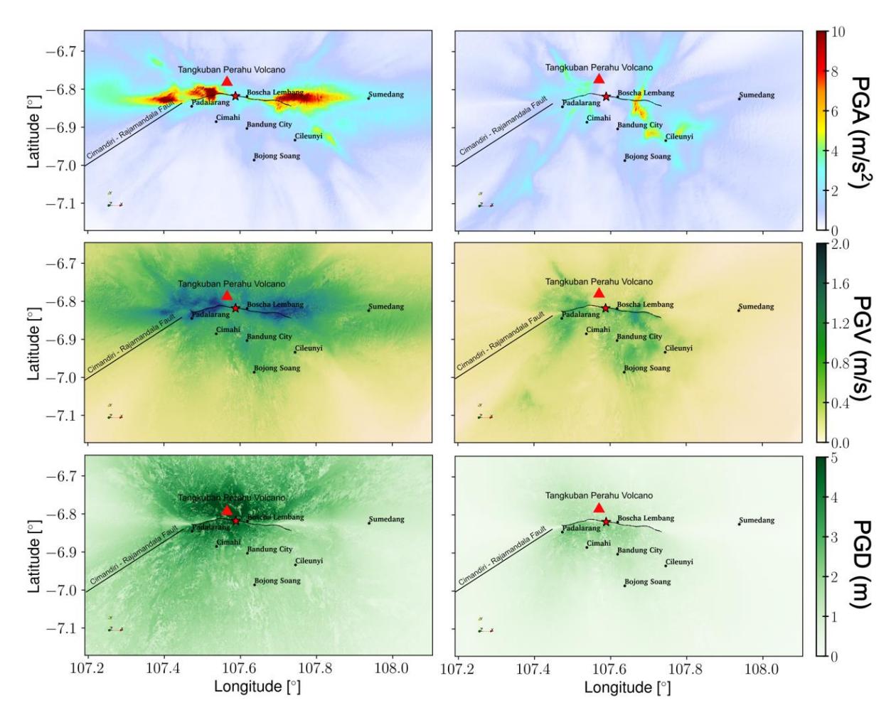
. Shakemaps for the two scenarios showing peak ground acceleration (PGA), peak ground velocity (PGV), and peak ground displacement (PGD). The maximum values are saturated at 10 m/s² for PGA, 2 m/s for PGV, and 5 m for PGD. The left panel shows the normal faulting scenario, while the right panel depicts the shakemap for the reverse faulting scenario.
From the two scenarios, normal faulting scenario (NFS) and reverse faulting scenario (RFS), we assessed the ground motion characteristics, including peak ground acceleration (PGA), peak ground velocity (PGV), and peak ground displacement (PGD) (Figure 6). The shakemaps exhibit very distinct characteristics. The left panel of Figure 6 depicts PGA from the NFS, showing strong shaking to the east and west of the Lembang Fault. Interestingly, the bending of the Lembang Fault (on both the western and eastern sides) produces rupture directivity, as indicated by high shaking exceeding 10 m/s². The affected areas include Boscha Observatory Lembang (4.8 m/s²), Sumedang (~3 m/s²), Padalarang (~2.8 m/s²), and Cileunyi (4.5 m/s²). In contrast, Bandung City, Cimahi, and Bojong Soang experience minimal shaking (< 1 m/s²). The right panel of Figure 6 shows a more widespread distribution of high PGA to the southern and northern areas, especially in Padalarang (2 m/s²), Cimahi (3 m/s²), Cileunyi (3.2 m/s²), and Bandung City (5 m/s²). However, areas with high shaking in the NFS, such as Sumedang, experience lower shaking in this scenario.
Both scenarios are realistic and verified against pre-existing ground motion models (GMMs). We compared the groundmotion intensity with GMMs from Boore et al. (2014), Campbell & Bozorgnia (2014), Abrahamson et al. (2014), and Idrissa (2014). Both GMMs are designed for large magnitudes (> 6), which aligns with our resulting seismic moment release. Each cell on the surface output is treated as a station, resulting in a total of 10 million stations. Figures 7a and 7b show the comparison between GMMs and synthetic data in relation to Joyner-Boore distance (the shortest distance from a site to the surface projection of fault planes) for the two scenarios. We used Joyner-Boore distance because of the considerably large extension and finiteness of the fault geometry (~25 km) as we are interested in the near-field region. Using hypocentral distance may mislead the comparison with the GMMs at the large slip located at further away from the hypocenter or epicenter. The median values of the synthetic data and GMMs are generally comparable, except for the RFS at distances less than 5 km, where the synthetic data underestimates the GMM predictions.
The PGV map shows how ground velocity varies along the fault line and its surroundings. High values are concentrated along the fault, particularly to the east and west of the hypocenter for the NFS. The highest shaking occurs near Padalarang, with PGV values exceeding 2 m/s. In the southern part of the Lembang Fault (e.g., Cimahi, Bandung City, Cileunyi, and Bojong Soang), the PGV values are relatively consistent, at approximately 1 m/s. In contrast, the RFS shows high PGV in the northern and southern parts of the Lembang Fault. However, the PGV values are lower than those in the NFS: Padalarang experiences shaking of 0.6 m/s, Cimahi 0.4 m/s, Bandung City 0.5 m/s, Bojong Soang 0.5 m/s, Cileunyi 0.5 m/s, and Sumedang 0.2 m/s.
The PGD map for the NFS shows that the highest displacements occur in the northern and southern parts of the Lembang Fault, indicating significant ground deformation. Notably, Padalarang exhibits deformations of up to 4.3 m and Cimahi up to 3.5 m. In the northern part of the Lembang Fault, deformation can reach up to 5.5 m. In the RFS, the highest shaking is located on the hanging wall of the Lembang Fault, specifically in the southern part, with PGD values exceeding 2.4 m in Padalarang. Similar to the PGV results, the shaking level in the RFS is smaller than in the NFS.
Pseudo-spectral acceleration (PSA) is a useful measure for the severity of the ground motion for structures in earthquake engineering. PSA plays a crucial role in estimating the peak response of a single-degree-of-freedom system (Baker et al., 2021). We evaluated three different PSA periods with 5% damping and has been verified with GMMs (Figure 7c and 7d); those are 0.1 s, 0.3 s, and 0.5 s (Figure 8). These values correspond to natural periods of buildings' height less than 7 m or 3 stories, larger building height is not considered here. For NFS (left panel in Figure 8), the affected areas are similar to PGA. Interestingly, PSA with a period of 0.5 s experiences high shaking up to 14 m/s2 to the eastern and western part of the Lembang Fault. In addition, high shaking also appears in the southeastern part of Cileunyi areas, which reaches a shaking level of ~11 m/s2 . For RFS, similar to the PGA map, high shaking is more widespread in the southern and northern areas (right panel in Figure 8), especially for higher periods, such as in Padalarang (6 m/s²), Cimahi (3.5 m/s²), Cileunyi (5 m/s²), and Bandung City (7 m/s²).
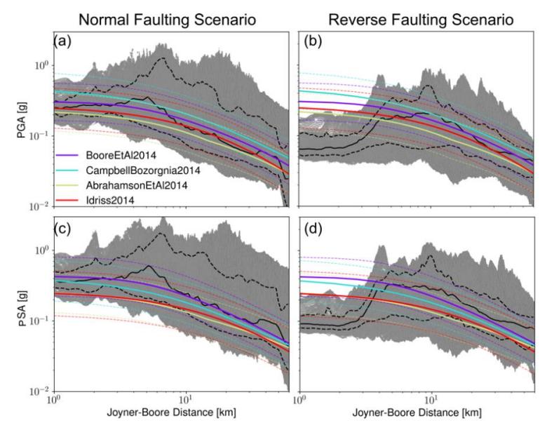
Comparison of the ground motion models (GMMs) from, Campbell & Bozorgnia (2014), Abrahamson et al. (2014), and Idrissa (2014) with the PGA (a and b) and pseudo-spectral acceleration (PSA for a period of 0.5 s with 5% damping, c and d) at each station versus Joyner-Boore distance. Each cell in the surface output from Figure 6 is considered a station. The black solid lines represent the median values of the synthetic data, while the dashed black lines indicate the 86th and 16th percentiles of the synthetic data. The solid-colored lines represent the median values of the GMMs, and the dashedcolored lines denote the standard deviation.
Discussions
Conditions leading to Mw 7
Our geometrically complex, 3D dynamic rupture simulations examine the feasibility of runaway self-sustained rupture on the Lembang Fault, constrained by the 3D geological structure. Based on our models, the two scenarios experience relatively similar conditions leading to destructive earthquakes despite differences in initial stress conditions and fault normal direction. Conditions leading to runaway self-sustained rupture, which result in a physically realistic stress drop, slip, maximum moment magnitude (7), and rupture duration, include relatively weak apparent strength (not optimally oriented and prestressed fault, with a lower ≈ 0.5 than 0 , subcritical stress, and overpressurized conditions. If these conditions are not met, we observed self-arrested ruptures with limited slip around the hypocenter (e.g., 0 < 0.75 and low ), leading to small magnitudes (< 4) or could grow to unrealistic earthquake source properties (e.g., 0 > 0.9 and very high ). Geometrical complexity also limits the slip extension, preventing it from breaking the entire fault plane. This complexity is characterized by two bends in the eastern and western parts of the Lembang Fault, resulting in a very low prestress ratio (< 0.3) (Palgunadi et al., 2024)), therefore limiting the slipping area.
Static and dynamic stress transfer to the Cimandiri-Rajamandala Fault
In the western part of the Lembang Fault, there is the Cimandiri-Rajamandala Fault, which strikes NE–SW. The static and dynamic stress transfers due to a rupture on the Lembang Fault could increase stress perturbations on the eastern side of the Cimandiri-Rajamandala Fault. Based on our results, the dynamic stress transfer is less than approximately 0.1 bar, whereas the static stress transfer exceeds 2 bars. Considering the magnitude of the stress transfer and the distance between the two faults (which is greater than 15 km), a dynamic rupture jump that could potentially activate rupture propagation at the tip of the Cimandiri-Rajamandala Fault is very unlikely. However, possibility of the activation owing to > 7 earthquake on the Lembang fault still arises in the long-term tectonic process. According to numerical experiments by Harris & Day (1993), the maximum distance over which one rupture can trigger another dynamic rupture is about 10 km. Although under very special stress conditions (such as a very weak and critically stressed fault) dynamic rupture jumping may occur over greater distances, as observed in the 2016 Kaikōura earthquake (Ulrich et al., 2019), this study does not explore such a scenario.
Distinct ground-motion pattern
Dynamic rupture in an earthquake strongly depends on the initial stress conditions, constitutive parameters (such as fault friction and physics at the rupture tip) on the fault, and fault geometry. Even when the hypocenter location, constitutive parameters, and fault geometry are the same, different initial stress conditions can lead to drastically different rupture dynamics. According to Palgunadi et al. (2024) and Gabriel et al. (2024), these differences primarily arise from distinct spatio-temporal slip evolution, stress drop, and static and dynamic stress interaction during the coseismic phase. Therefore, under different fault geometries and stress conditions, one may expect distinct rupture evolutions and, consequently, different ground motion distributions.
Our numerical experiments show that the two scenarios have different rupture characteristics and ground-motion patterns. The normal faulting scenario (NFS) is characterized by a slower average rupture speed (0.8 ), higher stress drop (12.8 MPa), and greater surface slip compared to the reverse faulting scenario (RFS). Interestingly, the RFS begins with slow rupture nucleation, but due to the higher overall prestress ratio (i.e., close to critical stress conditions), the rupture front develops into a supershear rupture. However, the rupture is confined below 1 km depth, leading to limited surface slip and a slip deficit at the fault bend, which could potentially reduce ground shaking. Although both scenarios consider normal and reverse faulting initial stresses, the source mechanisms still indicate a tendency toward strike-slip faulting, as reflected by the low up-dip or down-dip rake directions.
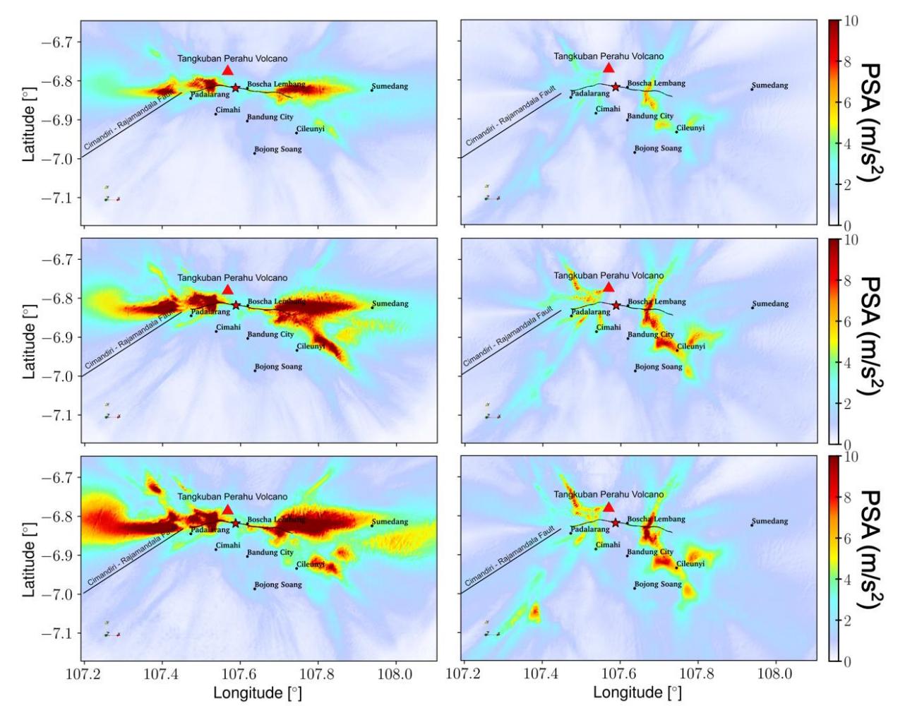
Shakemaps of the pseudo-spectral acceleration (PSA) with 5% damping for the two scenarios. The color scale is saturated at a maximum PSA of 10 m/s². The left panel shows the normal faulting scenario, while the right panel depicts the PSA for the reverse faulting scenario. The first, second, and third rows represent PSA with periods of 0.1 s, 0.3 s, and 0.5 s, respectively.
The ground-shaking patterns and amplitudes of the two scenarios are significantly distinct, mainly because of the spatiotemporal evolution of the slip and static-to-dynamic stress interaction between fault, bulk material, and surface topography. The affected areas and their shaking levels are contrasting: the NFS predominantly spreads to the east and west, while the RFS shows high shaking in the northern and southern parts of the Lembang Fault. These two scenarios highlight the importance of physics-based numerical simulations in assessing areas of high shaking that could result in massive destruction.
Limitations
The limitations of this study constrained from the lack of detailed knowledge of material and frictional properties, the assumption of relatively smooth stress distribution on the fault, and the use of a large-scale resolution of velocity model around the Lembang Fault. The assumed parameters for the dynamic rupture simulations may lead to distinct spatiotemporal slip evolutions and static-dynamic stress interactions, resulting in different ground motion distributions. Therefore, all the results presented in this study should be interpreted considering these assumed parameters.
Due to the high computational cost of each simulation, the results of this study are limited to only two scenarios and 40 dynamic simulations. This study is also limited to the geometrical details, 3D velocity structures, and initial stress conditions considered here. These scenarios investigate the significance of the unique fault geometry of the Lembang Fault, including dip direction, as indicated by previous studies. The geometrical complex of the Lembang Fault is supported by actual geological observations which suggest many small fault branches and segmentations.
Our study is also limited by the number of explorations regarding hypocenter location. The hypocenter location can significantly affect slip distribution, especially in the presence of geometric discontinuities like those in the Lembang Fault, e.g., study from Húsavík-Flatey fault zones (Li et al., 2023). Additionally, this study does not consider aseismic and poroelastic processes, which may contribute to rupture dynamics and, consequently, the resulting seismic moment and conditions leading to self-sustained rupture.
Conclusions
We present two main hypothetical earthquake scenarios for the Lembang Fault, which features a complex geometry. These two fault geometries primarily differ in their fault normal directions. To investigate conditions leading to a destructive earthquake, we assess scenarios within transitional regimes from normal to strike-slip faulting and from reverse to strike-slip faulting.
Conditions leading to runaway, self-sustained rupture are characterized by relatively weak apparent strength (i.e., a fault that is not optimally oriented and pre-stressed), subcritical stress, and overpressurized conditions. Under these conditions, earthquakes of magnitude > 7 can be generated. If these conditions are not met, we observe selfarrested ruptures that lead to smaller magnitudes ( < 4) or that could evolve into unrealistic earthquake source properties.
Ground motion patterns and amplitudes differ significantly between the two scenarios, mainly due to the spatiotemporal evolution of slip and the static-to-dynamic stress interactions among the fault, surrounding bulk material, and surface topography. In the scenario representing a transition from normal to strike-slip faulting, areas experiencing high ground motion (exceeding a peak ground acceleration of 1g) are predominantly located east and west of the Lembang Fault. In contrast, for the scenario transitioning from reverse to strike-slip faulting, the strongest ground shaking is primarily distributed north and south of the Lembang Fault.
It is important to note that this study explores scenarios that could lead to a worst-case event with the assumed initial conditions, resulting in a magnitude > 7.0 earthquake, posing a significant threat to the densely populated nearby city. Therefore, our findings have crucial implications for seismic hazard assessment around the Lembang Fault and necessitate further investigation to refine the physics-based model and different scenarios, for instance different hypocenter location and detailed shallow velocity structure.
Acknowledgment
The authors gratefully acknowledge financial support from the Institut Teknologi Sepuluh Nopember for this work, under the Capacity Development Program of Higher Education for Technology and Innovation Project Asian Development Bank Loan No 4110-INO. We also acknowledge financial support from Universitas Indonesia with contract number NKB-771/UN2.RST/HKP.05.00/2024 and from Universitas Gadjah Mada with contract number 1920/UN1/DITLIT/PT.01.03/2024. We thank three anonymous reviewers for the constructive comments and suggestions which help us to improve the manuscript. We also thank editor in chief Endra Gunawan, and associate editor Khoiruddin for handling the manuscript. Numerical simulations were performed on the ETH Zürich Euler cluster. Figures were prepared using Paraview (Ahrens et al., 2005) and Matplotlib(Hunter, 2007).
Compliance with ethics guidelines
The authors declare that they have no conflict of interest or financial conflicts to disclose.
This article does not contain any studies with human or animal subjects performed by any of the authors.