
Introduction
Given the dynamics of today's workforce, competent workers—especially engineers—are frequently tempted by fascinating offers at rival companies, creating an ongoing challenge for businesses dealing with high employee turnover. This phenomenon not only squanders invaluable talent but also burdens companies with exorbitant costs associated with recruiting and training new staff (Hashim, 2015). A study concluded that financial or non-financial motivation plays a pivotal role in enhancing job satisfaction among employees (Ali & Anwar, 2021). Defined by individuals' sentiments towards their work, job satisfaction permeates every aspect of their professional and personal lives, influencing their motivation and future performance. However, the problem of job satisfaction assumes greater importance in the field of civil engineering, which is distinguished by its technical complexity and dynamic working settings. The rapid pace of the construction sector, coupled with the inherent lack of control experienced by site-based engineers, calls for urgent attention to mental health considerations (ASCE, 2008; Haydam & Smallwood, 2016). Despite these pressing concerns, the transportation sector in Bagmati Province, Nepal, remains largely uncharted territory in terms of research and development.
An employee's motivation to perform well and want to stay with the company is fueled by their level of job satisfaction (Ali & Anwar, 2021). Because of its fast-paced construction industry and strict technical specifications, civil engineering poses unique challenges, particularly for employees stationed on construction sites. Engineers frequently struggle with uncontrollable situations and increasing work expectations, which highlights the importance of putting their mental health first. Motivation theorists discuss both extrinsic and intrinsic motivators. Interest, challenge, and self-satisfaction
are examples of intrinsic motivators that inspire someone to take action on their own. Pay, bonuses, and other material benefits that originate from sources outside of the individual are examples of extrinsic motivators (Pandya, 2024).
The urban areas in Nepal are growing very fast due to the relatively greater economic and educational opportunities compared to rural areas (Bhattarai et al., 2023). The Bagmati Province, in the central region and the capital Kathmandu, has obvious construction and substantial investments in infrastructure with significant expansions in the road network that exists within the province. Given these developments, the job satisfaction of civil engineers operating within the transportation sector of Bagmati Province is crucial for ensuring the smooth implementation of transportation projects. By examining the job satisfaction levels of civil engineers within the transportation sector, the study aims to identify key influencing factors and suggest actionable strategies for enhancement. To that end, this study addresses the research question: "1) What factors influence job satisfaction among civil engineers in the transportation sector of Bagmati Province, Nepal; 2) how do they impact job performance; 3) how do they vary between private and government employment; and 4) what are the potential remedial measures?
To achieve these objectives, the study applies Principal Component Analysis (PCA) to reduce data complexity and Structural Equation Modeling (SEM) to map the interrelations among influencing variables. These combined methods offer a deeper understanding of the satisfaction drivers within the civil engineering domain: SEM maps the links between the key dimensions that PCA emphasizes, offering profound insights into the dynamics of satisfaction in the civil engineering profession.
Literature Review
The Single Global Rating Method (SGRM) answers a single question: "In general, how satisfied are you with your job?" On a scale from "very satisfied" to "very dissatisfied," respondents are asked to circle their preferred response. The second method is the Summation Job Factor Method (SJFM), which is more advanced as it describes a job's duties, supervision, pay, advancement possibilities, and co-workers. Researchers collect responses on a standardized scale for each of these and then combine the results to provide an aggregate measure of employee satisfaction in the workplace (Robbins & Judge, 2013).
Research by Bhatta et al. (2018) on 44 civil engineers employed in Nepal's construction sector revealed high overall job satisfaction, with notable links between satisfaction and factors like annual income and work experience. Gender and location, however, did not significantly affect satisfaction levels. Engineers were particularly satisfied with their team dynamics and job nature but expressed discontent with salary structures, promotion opportunities, and working conditions. Another study conducted by Paudel et al. (2020) among 103 civil engineers in Gandaki Province reported general satisfaction with job roles, but dissatisfaction with salary and advancement paths remained prominent concerns. Their regression analysis demonstrated that about 58.2% of the variability in job satisfaction could be explained by supervisory support, peer relationships, promotion prospects, compensation, and transfer policies. In the hydropower consultancy sector, Thapa and Shrestha (2018) found that although civil engineers generally expressed job satisfaction, remuneration and promotion systems remained points of discontent. Their findings, based on descriptive and inferential statistics, emphasized that job nature, supervisor relationships, work conditions, and advancement opportunities were critical satisfaction drivers. Similarly, Paudel et al. (2019) investigated civil engineers in Nepal's irrigation sector and found that while many were satisfied overall, dissatisfaction was again centered on promotion and compensation systems. The study also identified that male engineers and those in office-based roles tended to report higher satisfaction than their female and site-based counterparts.
The study examines Jordanian construction engineers' work satisfaction characteristics to develop a model. The working environment, colleague relationships, remuneration and perks, and supervision all greatly affect job satisfaction. The model, substantiated by interviews, shows how employment happiness boosts construction company production. Also important is cultural background on contentment. The study emphasizes the role of workload, work environment, and salary in engineers' happiness and offers solutions for improving teamwork and safety (Alzubi et al., 2023). The culture of an organization has a big effect on how happy employees are with their jobs. Organizational culture, balance between life and work, and satisfaction with job all make people more engaged at work. People who are happy with their jobs and have a good work-life balance are more engaged. It helps shape employee behavior, fostering commitment, which further enhances organizational success. A strong organizational culture fosters ownership, leading to increased employee participation (Perkasa et al., 2023; Rivai & Syahril, 2024; Suriyanti, 2024).
A study examines the connection between employee performance and job satisfaction in Pakistan's construction sector, highlighting important variables that affect both. The study outlines 11 parameters that contribute to job satisfaction, including aspects like compensation, promotions, and the work environment, as well as eight criteria for evaluating employee performance, which encompass teamwork, problem-solving, and time management. The findings indicate that elements such as compensation, incentives, job stability, and secure work environments play a significant role in influencing satisfaction with jobs, whereas the knowledge and skills of employees are essential for performance outcomes. The research highlights the importance of organizations concentrating on these elements to boost job satisfaction and employee performance, ultimately resulting in greater productivity and efficiency within the construction industry. The findings, which were looked at with the Relative Importance Index (RII) and SPSS, give us important ideas for how to manage human resources better in the future (Memon et al., 2023).
A study carried out with high school teachers in Laguna, Philippines, revealed that although work-life balance and motivation had minimal impact on job commitment, job satisfaction significantly contributed to it positively. Factors such as age and experience served as moderating influences, with teachers who were older and more experienced demonstrating greater levels of commitment. In a similar vein, the study conducted at PT Sucofindo Makassar Branch in Indonesia indicated that both the balance between work and life with the work environment had a big effect on job satisfaction, with the balance alone explaining 91.2% of the variance. While employees expressed overall satisfaction with the work environment, they highlighted specific areas that could benefit from enhancements, particularly in the management of work-life balance and the dynamics with their superiors. Both studies highlight the significance of enhancing job satisfaction to improve commitment and achieve overall organizational success (Amin & Sudiana, 2024; Munda & Gache, 2024).
Methodology
This research focused on Bagmati Province as its primary subject area. Bagmati Province is home to the country's capital city, Kathmandu, and several other major cities like Lalitpur, Bhaktapur, and Kavre. The province covers an area of 20,300 square kilometers. The study identified all civil engineers in the transportation sector of Bagmati Province as the focal population. 134 engineers voluntarily participated in this study, and the researcher distributed a Google Form questionnaire via email to gather respondents. In other words, access to respondents is based on their availability and desire to engage. Because of this, the resulting sample was self-selected.
Sample Size
The following formula was employed to determine the sample size (Cochran, 1977):
\[n_o = \frac{z^2 p q}{e^2}\] where (no) refers to the sample size for an infinite population, (z) is the critical value of the desired confidence level, (p) is the estimated proportion of an attribute that is present in the population; q=1-p, (e) represents the desired level of precision. Hence, by using the formula above, the calculated sample size for the study is presented below.
\[n_o = \frac{1.96^2 \times 0.5 \times 0.5}{0.085^2} = 132.93\]
The survey requires a sample of 132.93 civil engineers based on Cochran's formula. The researcher received only 134 valid responses out of the 150 distributed questionnaires. A total of 89.33% of the responses obtained were considered valid and were duly recorded. We used MSQ for the Summation Job Facet Method.
SEM is a statistical approach used for confirmatory analysis of structural theories related to various phenomena. The method entails procedures that examine cause and effect by analyzing observations on various constructions. SEM is better than multiple regression when it comes to modeling interactions, correlated independents, nonlinearities, correlated error terms, and multiple latent independents, each of which is measured by more than one scale.SEM provides numerous benefits, such as handling intricate variable relationships, identifying overlooked indicators, and estimating all coefficients in the model at once. This thorough analysis enables researchers to evaluate the significance and strength of relationships comprehensively. SEM also lets you do statistical analysis of proposed conceptual models to make sure they match the data by looking at the whole variable or construct structure at the same time (Sukamani et al., 2021; Wu et al., 2015). Many previous researchers have used SEM models specific to the construction management field (Falce et al., 2023; Kineber et al., 2021; Liu et al., 2020).
As an adaptive method of data analysis, principal component analysis (PCA) reduces the number of variables in datasets, making them easier to understand while minimizing information loss by generating new, uncorrelated variables that sequentially maximize variance; these new variables, known as principal components, are derived by solving an eigenvalue/eigenvector problem. The specific dataset being analyzed dictates these new variables, making PCA an adaptive method of data analysis (Jolliffe & Cadima, 2016). Many past job satisfaction studies used PCA analysis in construction projects (Adekunle et al., 2022; Aung et al., 2023; Ingle & Mahesh, 2022).
MSQ was used to obtain comprehensive data on job satisfaction, providing a structured foundation for analysis. PCA was selected to simplify the data by identifying the most significant factors that contribute to job satisfaction. This approach helps streamline the analysis while preserving essential information. SEM was used to examine and model the relationships between these factors, providing a deeper understanding of how they interact and influence job satisfaction. Finally, MDM was applied to manage uncertainty in responses, capturing varying degrees of satisfaction more accurately. These methods complement each other by sequentially addressing data collection, dimensionality reduction, relationship modeling, and response uncertainty, ensuring a thorough and reliable analysis.
Hypothesis
Based on prior research, the following hypotheses were developed:
- 1. Hypothesis T1: Job performance and work culture exhibit a positive and substantial correlation.
- 2. Hypothesis T2: Job performance and work-life balance exhibit a positive and substantial correlation.
- 3. Hypothesis T3: Job performance and employee engagement are significantly and positively correlated.
Data Analysis
The demographic profiles of the respondents are shown in Table 1.
Table 1 Profile of respondent.
| Category | Sub-Categories | Frequency | Percent |
|---|---|---|---|
| Gender | Male | 118 | 88.10 % |
| Female | 16 | 11.90 % | |
| Total | 134 | 100.0 % | |
| less than 25 | 18 | 13.40 % | |
| 26-30 | 64 | 47.80 % | |
| Age Group | 31-35 | 28 | 20.90 % |
| more than 36 | 24 | 17.90 % | |
| Total | 134 | 100.0 % | |
| Bachelor | 72 | 53.70 % | |
| Highest Qualification | Master | 62 | 46.30 % |
| Total | 134 | 100.0% | |
| 1 or less | 18 | 13.40 % | |
| 2-5 | 52 | 38.80 % | |
| Total Work Experience | 6-10 | 40 | 29.90 % |
| 11-20 | 10 | 7.50 % | |
| more than 21 | 14 | 10.40 % | |
| Total | 134 | 100.0 % | |
| 1 or less | 40 | 29.90 % | |
| Work Experience in | 2-5 | 66 | 49.30 % |
| Current Organization | 6-10 | 16 | 11.90 % |
| more than 11 | 12 | 9.00 % | |
| Total | 134 | 100.0 % | |
| Office | 46 | 34.30 % | |
| Job-Based on | Site | 12 | 9.0 % |
| Both | 76 | 56.70 % | |
| Total | 134 | 100.0 % | |
| Government | 46 | 34.30 % | |
| Job Type | Private | 88 | 65.7 % |
| Total | 134 | 100.0 % | |
The analysis of the responses received revealed that the mean scores for intrinsic, extrinsic, and general satisfaction are 45.51, 19.06, and 64.57, respectively. The corresponding percentile scores for these three categories of satisfaction are 27.55, 30.30, and 10.71, respectively. A score of 75 or higher indicates a high level of contentment, while a score of 25 or less indicates a low level of satisfaction. A moderate degree of contentment is indicated by scorers between 26 and 74 (Weiss et al., 1967). This criterion indicates that the sample group has low levels of overall work satisfaction but average levels of extrinsic and intrinsic job satisfaction.
| Job Satisfaction | Frequency | Percent |
|---|---|---|
| Very Dissatisfied | 10 | 7.5 % |
| Dissatisfied | 32 | 23.9 % |
| Neither (Dissatisfied nor satisfied) | 50 | 37.3 % |
| Satisfied | 26 | 19.4 % |
| Very satisfied | 16 | 11.9 % |
| Total | 134 | 100.0 % |
Table 2 JS based on SGRM (Single Global Rating Method).
Additionally, based on the SGRM results presented in Table 2, the researcher obtained an average score of 3.04 out of 5, which suggests that the sample group is "somewhat satisfied" when directly questioned about their job satisfaction. The summation job factor method is more advanced than the single global rating method because it explains all the other variables (Robbins & Judge, 2013). So, the researcher used the summation method to assess job satisfaction and found that civil engineers working in the transportation sector of Bagmati Province have a low level of job satisfaction. The study of the job satisfaction of civil engineers in irrigation, building, hydropower, and Gandaki Province also concluded that civil engineers are somewhat satisfied with their jobs but are dissatisfied with the pay/salary and promotion opportunities (Bhatta et al., 2018; Paudel et al., 2019; Paudel et al., 2020; Thapa & Shrestha, 2018).
SPSS Testing and Result
The Kaiser-Meyer-Olkin (KMO) measure was used to assess whether the data was sufficient for factor analysis. To evaluate if the dataset is appropriate for factor analysis, several analyses are performed, including the determinant score, correlation matrix, and Bartlett's test of sphericity (Shrestha, 2021). The KMO test assesses data for factor analysis and sample size. It uses the KMO and Bartlett's tests of sphericity to validate the PCA. KMO values range from 0.8-1.0 for sufficient sampling to 0.6 for inadequate sampling. Acceptable values range from 0.5 to 0.6 for 100 to 200 samples. The Bartlett's test results, with a significance level of p<0.001, suggest strong relationships among factors in the correlation matrix, indicating the potential of factor analysis (FA) for the data set, as indicated by the 2472.973 test result. (Shrestha, 2021). The factor number was found to be KMO value 0.829; Bartlett value χ2 = 2472.973; df = 276 (p=.00); the scale has 24 items. Table 3 shows that the KMO statistics value of 0.829 indicates that the sampling and factor analysis for the data are reliable.
Measure of Sampling Adequacy (Kaiser-Meyer-Olkin) 0.829 Bartlett's Test of Sphericity Approx. Chi-Square 2472.97 Degree of freedom 276 Significant 0.00
Table 3 Test Result of KMO and Bartlett.
Factor Extraction
The study used the eigenvalue method to find the best number of elements to extract (Shrestha, 2021). Given the circumstances, only factors with eigenvalues greater than 1.0 were kept. Varimax was used for normalization to reduce the complexity of the factors and maximize the model's variance. The scree plot is an effective instrument for identifying the ideal number of factors to retain in exploratory FA for PCA. The scree plot shows that four factors have eigenvalues greater than one and explain most of the data variation. Very little of the difference comes from the other factors, which aren't thought to be as important (Shrestha, 2021).
PCA suggested that more than 50% of the total variation should be explained by the factors that are kept. The findings, as presented in Table 4, show that four factors explain 66.315% of the variance (Chanda et al., 2023). The KMO value of 0.829 indicates adequate sampling adequacy, suggesting that factor analysis is beneficial for the variables. In the study's scope, it was found that there are four factors with an eigenvalue of more than 1.
Table 4 Explanation of Eigen Values (EV) and Total Variance.
| Component | Initial Eigenvalues | Extraction Sums of Squared Loadings | Rotation Sums of Squared Loadings | ||||||
|---|---|---|---|---|---|---|---|---|---|
| Percentage | Cumulative | Percentage | Cumulative | Percentage | Cumulative | ||||
| Aggregate | of Variance | Percentage | Aggregate | of Variance | Percentage | Aggregate | of Variance | Percentage | |
| 1 | 10.34 | 43.10 | 43.10 | 10.34 | 43.10 | 43.10 | 6.93 | 28.88 | 28.88 |
| 2 | 3.02 | 12.58 | 55.68 | 3.02 | 12.58 | 55.68 | 3.41 | 14.23 | 43.11 |
| 3 | 1.38 | 5.77 | 61.46 | 1.38 | 5.77 | 61.46 | 2.91 | 12.15 | 55.26 |
| 4 | 1.16 | 4.85 | 66.31 | 1.16 | 4.85 | 66.31 | 2.65 | 11.05 | 66.31 |
| 5 | 0.99 | 4.13 | 70.44 | ||||||
| 6 | 0.84 | 3.51 | 73.96 | ||||||
| 7 | 0.80 | 3.35 | 77.31 | ||||||
| 8 | 0.70 | 2.91 | 80.23 | ||||||
| 9 | 0.64 | 2.67 | 82.91 | ||||||
| 10 | 0.58 | 2.44 | 85.36 | ||||||
| 11 | 0.51 | 2.13 | 87.49 | ||||||
| 12 | 0.46 | 1.93 | 89.42 | ||||||
| 13 | 0.41 | 1.73 | 91.16 | ||||||
| 14 | 0.37 | 1.54 | 92.70 | ||||||
| 15 | 0.32 | 1.36 | 94.07 | ||||||
| 16 | 0.31 | 1.29 | 95.36 | ||||||
| 17 | 0.22 | 0.94 | 96.30 | ||||||
| 18 | 0.19 | 0.83 | 97.13 | ||||||
| 19 | 0.17 | 0.74 | 97.87 | ||||||
| 20 | 0.17 | 0.71 | 98.59 | ||||||
| 21 | 0.10 | 0.43 | 99.02 | ||||||
| 22 | 0.09 | 0.37 | 99.39 | ||||||
| 23 | 0.07 | 0.30 | 99.70 | ||||||
| 24 | 0.07 | 0.29 | 100.00 |
Extraction method : PCA
Factor Rotation and Interpretation
Cronbach's alpha tests instrument accuracy and reliability by confirming internal consistency. The Cronbach's alpha value should exceed 0.7 (Gefen et al., 2000). Table 6 confirms the survey's reliability. The variables are internally consistent since they correlate with their component grouping. This study identified only twenty out of the twenty-four items for job satisfaction as major components. The researcher categorized all these components into four parts through Principal Component Analysis, as presented in Table 5.
Table 5 Rotated Component Matrix.
| Component | ||||
|---|---|---|---|---|
| Variables | WC | WLB | EE | JSE |
| IM8 | 0.83 | |||
| IM10 | 0.76 | |||
| IM7 | 0.71 | |||
| EM6 | 0.70 | |||
| IM9 | 0.70 | |||
| EM2 | 0.70 | |||
| IM13 | 0.67 | |||
| IM11 | 0.63 | |||
| EM3 | 0.61 | |||
| WL2 | 0.91 | |||
| WL1 | 0.89 | |||
| WL3 | 0.88 | |||
| WL4 | 0.65 | |||
| IM3 | 0.82 | |||
| IM2 | 0.65 | |||
| IM6 | 0.61 | |||
| EM5 | 0.80 | |||
| Extraction Method: PCA |
Rotation Method: Varimax with Kaiser Normalization in 6 iterations.
Table 6 Cronbach's Alpha
| Component | Cronbach's Alpha |
|---|---|
| WC | 0.92 |
| WLB | 0.74 |
| EE | 0.87 |
Component 1: Work Culture - This component contributed to 43.101% of the overall variance with an Eigenvalue of 10.344. It is the set of shared values, beliefs, attitudes, and practices that shape staff behaviour and experiences. Independence, creativity, variety, ethical culture, and fair policies can enhance job satisfaction and commitment(Amabile, 1997; Baer & Frese, 2003; Davis & Rothstein, 2006; Kristof‐Brown et al., 2005; Mayer et al., 2010). In summary, establishing an ethical and fair work culture will help to produce a more pleasant workplace and improved results for staff members. Component 2: Work-Life Balance - This term accounted for 12.587% of the overall variance, with an Eigenvalue of 3.021. It has a substantial impact on job satisfaction, and flexible working hours may help reduce conflict between work and personal life (Allen et al., 2000; Ernst Kossek & Ozeki, 1998). Component 3: Employee Engagement - This aspect contributed to 5.772% of the overall variance, with an Eigenvalue of 1.385. Understanding individuals' degree of commitment and connection to their work, organization, and colleagues can be influenced by different elements such as job satisfaction, feeling of progress, and support from coworkers. (Bakker & Leiter, 2010; Eisenberger et al., 2001; Harter et al., 2002). Component 4: Job Security - This element accounted for 4.855% of the overall variance, with an Eigenvalue of 1.165. Job satisfaction is higher in employees who perceive their jobs as secure, while job insecurity can lead to negative emotions like anxiety, depression, and frustration, negatively impacting health and well-being. (Reisel et al., 2010).
PLS-SEM Model Testing and Result
The single variable identified by the PCA is the only indicator of the construct of interest; it may not be sufficient to establish construct validity and reliability (Santos, 1999). As a result, it was eliminated so that the researcher could conduct a more accurate analysis.
Measurement Model's Validity and Reliability
Assessing the validity and reliability of the measurement model is one of the first steps in PLS analysis. Cronbach's alpha (CA), Composite Reliability (CR), Average Variance Extracted (AVE), and indicator loading are displayed in Table 7. When the loading number was higher than 0.7, it showed reliability (Hulland, 1999). In the same way, the CR and CA of all the model's builds were above 0.7, which shows that they are reliable (Gefen et al., 2000). All of the constructs have an AVE above 0.5, which indicates that they are all valid (Bagozzi & Yi, 1988; Fornell & Larcker, 1981b). The study also utilized Fornell and Larcker criteria, the Heterotrait Monotrait Ratio (HTMT), and cross-loadings to assess the discriminant validity (Sukamani et al., 2020). The abbreviations for the items are provided in Appendix.
Table 7 Indicator and Convergent Validity
| Elements | Loading | CA | CR | AVE | |
|---|---|---|---|---|---|
| IM2 | 0.87 | ||||
| EE | IM3 | 0.90 | 0.88 | 0.92 | 0.81 |
| IM6 | 0.92 | ||||
| EM2 | 0.88 | ||||
| EM3 | 0.44 | ||||
| EM6 | 0.78 | ||||
| IM10 | 0.85 | 0.92 | 0.59 | ||
| WC | IM11 | 0.47 | 0.90 | ||
| IM13 | 0.85 | ||||
| IM7 | 0.84 | ||||
| IM8 | 0.82 | ||||
| IM9 | 0.81 | ||||
| JP1 | 0.92 | ||||
| JP | JP2 | 0.92 | 0.89 | 0.93 | 0.82 |
| JP3 | 0.87 | ||||
| WL1 | 0.90 | ||||
| WL2 | 0.88 | ||||
| WLB | WL3 | 0.90 | 0.92 | 0.94 | 0.81 |
| WL4 | 0.91 |
In Table 8, you can see that all of the consistent manifest variables have higher values than their corresponding latent variables when the cross-loadings are taken into account. The salient feature in the diagonal indicates item cross-loading inside its framework (Chin & Marcoulides, 1998; Chin, 2009).
Table 8 Discriminant Validity; Indicator Items Cross
| EE | JP | WC | WLB | |
|---|---|---|---|---|
| EM2 | 0.21 | 0.45 | 0.88 | 0.27 |
| EM3 | 0.30 | 0.42 | 0.44 | 0.30 |
| EM6 | 0.23 | 0.29 | 0.78 | 0.13 |
| IM10 | 0.18 | 0.39 | 0.85 | 0.15 |
| IM11 | 0.36 | 0.40 | 0.47 | 0.30 |
| IM13 | 0.22 | 0.46 | 0.85 | 0.24 |
| IM2 | 0.87 | 0.34 | 0.15 | 0.17 |
| IM3 | 0.90 | 0.42 | 0.25 | 0.24 |
| IM6 | 0.92 | 0.47 | 0.37 | 0.35 |
| IM7 | 0.15 | 0.35 | 0.84 | 0.20 |
| IM8 | 0.19 | 0.38 | 0.82 | 0.12 |
| IM9 | 0.16 | 0.39 | 0.81 | 0.20 |
| JP1 | 0.47 | 0.92 | 0.50 | 0.50 |
| JP2 | 0.43 | 0.92 | 0.48 | 0.43 |
| JP3 | 0.34 | 0.87 | 0.46 | 0.29 |
| WL1 | 0.27 | 0.44 | 0.29 | 0.90 |
| WL2 | 0.24 | 0.34 | 0.20 | 0.88 |
| WL3 | 0.28 | 0.42 | 0.31 | 0.90 |
| WL4 | 0.25 | 0.44 | 0.25 | 0.91 |
The HTMT correlation ratio between model constructs is indicated in Table 9 to be less than 0.9, which is below the threshold (Henseler et al., 2009).
Table 9 Discriminant Validity (Htmt)
| EE | JP | WC | WLB | |
|---|---|---|---|---|
| EE | ||||
| JP | 0.51 | |||
| WC | 0.32 | 0.58 | ||
| WLB | 0.31 | 0.49 | 0.31 |
The square root of each concept's AVE numbers and their correlations are displayed in Table 10. Because they are greater than the association coefficients with other constructs, the square roots of the AVE, which are shown by the numbers in bold, passed the discriminant validity test. The latent variable with the highest values across all rows and columns is displayed in Table 10 as the square root of the AVE. The numbers show how this construct relates to other structures outside of the bolded diagonals (Fornell & Larcker, 1981a).
Table 10 Discriminant Validity (Fornell and Larker Criteria)
| EE | JP | WC | WLB | |
|---|---|---|---|---|
| EE | 0.90 | |||
| JP | 0.46 | 0.90 | ||
| WC | 0.30 | 0.53 | 0.76 | |
| WLB | 0.29 | 0.46 | 0.29 | 0.90 |
Evaluation of Structure Model
Collinearity testing and path coefficient determination were carried out as part of the structural model's study and validation. Since all VIF values are less than 5, there is neither a strong suggestion of multicollinearity nor its absence (Cassel et al., 1999; Hair et al., 2011). The collinearity analysis result is displayed in Table 11. Multicollinearity in the structural equation model was evaluated by inspecting the values of the inner VIF. All VIF values were under 5; hence, multicollinearity was not an issue (Henseler et al., 2009).
Table 11 Result of Collinearity Assessment
| Predictor construct | Endogenous Variable | Variance Inflation Factors (VIF) |
|---|---|---|
| EE | Effect of JP | 1.16 |
| WC | Effect of JP | 1.16 |
| WLB | Effect of JP | 1.15 |
Table 12 Hypothesis Testing in the Structural Model (Direct)
| Hypo thesis | Relationship | Beta | LLCI (2.5%) | ULCI (97.5%) | T Statistics (|O/STDEV|) | P Values | Decision |
|---|---|---|---|---|---|---|---|
| T1 (a) | WC -> JP | 0.37 | 0.21 | 0.51 | 4.86 | 0.000 | Supported |
| T2 (b) | WLB -> JP | 0.27 | 0.11 | 0.45 | 3.10 | 0.002 | Supported |
| T3 (c) | EE -> JP | 0.27 | 0.12 | 0.41 | 3.40 | 0.001 | Supported |
The path coefficient demonstrates how changing the predictor construct by one influence the endogenous construct. Beta value examines all latent variables. Beta values increase as exogenous (predictor) variables have a greater effect on endogenous variables (Aibinu & Al-Lawati, 2010). Using the t-test, the beta is calculated. For determining the t-value, non-parametric bootstrapping is employed. Bootstrapping uses a specified number of tests to calculate the t-value. Bootstrapping generated 5000 samples for t-value calculations (Henseler et al., 2009; Hoonakker et al., 2010). For a two-tailed test (t-value >= 1.96 at p = 0.05, 2.58 at 0.01, and 3.29 at 0.001), pioneers held the following beliefs (Hair et al., 2011). The same threshold values were used. Table 12 reveals that all paths had t-values over 1.96 at 5% significance. The highest beta value was 0.372, which shows that the effects of work culture on job performance are highly related.
Model fit test showed all parameters were within optimal range, exceeding threshold levels. Both the measurement and structural models were reliable and valid. The results of all three hypothetical scenarios (T1-T3) in Table 12 underscore the significance of the SEM model. One direct hypothesis (T3) was supported at a 5 % significance level, and two direct hypotheses (T1 and T2) were supported at a less than 1% significance level, as indicated in Table 12.
Work Culture: - After conducting a thorough analysis, it was found that the relation between work culture and job performance stood out as the most significant among all other factors, with a t-value of 4.86 and a beta value of 0.37. Having a positive work environment can result in increased job satisfaction, productivity, and performance (Ameer, 2017). Organizational culture plays a significant role in fostering organizational commitment, which in turn enhances job performance. (Hlaing, 2019; Parashakti et al., 2020). Employee Engagement - It has been shown to have a statistically significant impact on job performance, with a t-value of 3.40 and a beta value of 0.27. Employee engagement has a substantial positive impact on job performance (Ismail et al., 2019). Good working relationships play a crucial role in producing high-quality work. Employee engagement affects job performance more than organizational commitment (Bacong & Encio, 2017; Dajani & Zaki, 2015). This evidence suggests that while employee engagement is crucial for job performance, other factors may play a role in fostering organizational commitment. Work-Life Balance – It demonstrated statistical importance to job performance, as indicated by a t-value of 3.10 and a beta value of 0.27. Job performance is influenced by achievement and work-life balance, particularly among millennials who have flexible hours and supportive supervision (Dousin et al., 2019; Duan & Deng, 2022; Wiradendi Wolor, 2020). These findings show that work-life balance and supportive workplaces boost employee engagement and performance.
Evaluation Process
The MDM principle is used to compare and rank different categories based on their level of job satisfaction. The matrix values reflect the proportion distribution of each indicator inside each construct, which is used to calculate the membership MDM. Details are provided below.
Evaluation Matrix
The gathered data is segmented into two sections: government and private. Further, data was assessed using three indicators of job satisfaction. The judgment level was used as in the questionnaire for the latent construction factor, which is represented by following Eq. (1):
\[K_{pq}^{cd}\] = (p=1,2,3; q=1,2,3; c=1,2; d=1,2,3,4,5) (1)
Where, In this case, "K" stands for the degree of membership, "p" denotes the number of an exogenous construct or factor that is assumed to have an independent effect on the outcome being studied, "q" denotes the number of indicators in each construct, "c" denotes different levels or types of a particular category, and "d" denotes the judgment
level from 1 (excellent) to 5 (very poor) (Sukamani & Wang, 2020; Sukamani et al., 2020). \(K_{pq}^{cd}\) was used to represent the proportional distribution of each indicator inside each construct, whereas Eq. (2) was used to determine the proportional distributions. The evaluation matrix for fraction distribution of the ith phase with the lth kind of job type was represented by \(K_p^c\) as given in Eq. (3). The vector \(K^c\) represents assessment data for every facet based on the \(c^{th}\) categories of job types.
\[K_{pq}^{cd} = \frac{a_{pq}^{cd}}{\sum_{n=1}^{5} a_{pq}^{cd}}, \text{ p=1,2,3; q=1,2,3; c=1,2; d=1,2,3,4,5}\] (2)
\[K_{p}^{c} = \begin{bmatrix} K_{p1}^{c1} & K_{p1}^{c2} & K_{p1}^{c3} & K_{p1}^{c4} & K_{p1}^{c5} \\ K_{p2}^{c1} & K_{p2}^{c2} & K_{p2}^{c3} & K_{p2}^{c4} & K_{p2}^{c5} \\ K_{p3}^{c1} & K_{p3}^{c2} & K_{p3}^{c3} & K_{p3}^{c4} & K_{p3}^{c5} \end{bmatrix}\] \[(3)\]
Weight Distribution
After making sure that both discriminant and convergent validity were supported, the PLS model's path coefficient and indicator loading values were used. \(\sigma_{mn}\)= (m=1, 2,3; n=1, 2, 3) displays the value of the loading indicator of the n<sup>th</sup> indicator in the m<sup>th</sup> form. The weight of the n<sup>th</sup> indicator in the m<sup>th</sup> indicator was represented by the symbol \(\beta_{mn}\), which was the determined value from the Eq. (4). Eq. (5) describes all m<sup>th</sup> indicators. Let \(z_m\) (m=1, 2,3) represent the path coefficient in the mth form where the m<sup>th</sup> form weight was represented by w<sub>i</sub>, produced by Eq. (6). Eq.(7) calculates all weight factors.
\[\beta_{mn} = \frac{\sigma_{mn}}{\sum_{k=1}^{6} \sigma_{mn}}, m=1,2,3; n=1,2,3\] (4)
\[B_i = \beta_i = [\beta_{i1} \beta_{i2} \beta_{i3}] \tag{5}\]
\[W_i = \frac{z_m}{\sum_{j=1}^5 z_m}\], m=1, 2, 3 (6)
\[W = [w_1 \ w_2 \ w_3] \tag{7}\]
Result
Concerning the evaluation matrix \(K_p^c\) and weight matrix \(B_i\), the comprehensive evaluation vector of the ith indicator related to the cth job type, \(Q_p^c\), was computed by Eq. (8). The comprehensive evaluation vector of the cth is \(R^c\), computed by Eq. (9). The MDM principle was used to assess the job satisfaction of civil engineers in the transportation industry (government or private job) by selecting the highest value from a five-level scale as the outcome. For instance, if \(R^c\) had values of (0.2, 0.3, 0.25, 0.27, and 0.28) across the spectrum of (excellent, good, fair, poor and very poor), it would be rated as II (good) since the value it had at the second level was the highest across all five levels.
\[Q_p^c = \beta_1 x K_p^c = [Q_p^{c1} Q_p^{c2} Q_p^{c3} Q_p^{c4} Q_p^{c5}], p=1,2,3; c=1, 2\] (8)
\[R^{C} = W \times \begin{bmatrix} Q_{p}^{C1} \\ Q_{p}^{C2} \\ Q_{p}^{C3} \\ Q_{p}^{C4} \\ Q_{p}^{C5} \end{bmatrix}\] (9)
Based on the above steps and Eq. (9), the researcher evaluated the job categories of civil engineers in the transportation industry according to their level of job satisfaction, as shown in Table 13 (Sukamani & Wang, 2020; Sukamani et al., 2020). The findings indicate that in the private sector, job satisfaction is II (poor), whereas in the government sector, job satisfaction is III (fair). Despite having a fair level of job satisfaction, government engineers exhibit poor employee engagement.
Table 13 Ranking Government and Private Job Type
| Excellent | Good | Fair | Poor | Very poor | |
|---|---|---|---|---|---|
| Private | 0.09 | 0.19 | 0.26 | 0.30 | 0.14 |
| Public | 0.11 | 0.17 | 0.34 | 0.29 | 0.06 |
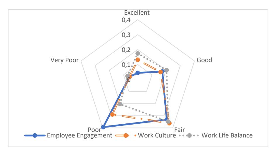
Evaluation result for government job type.
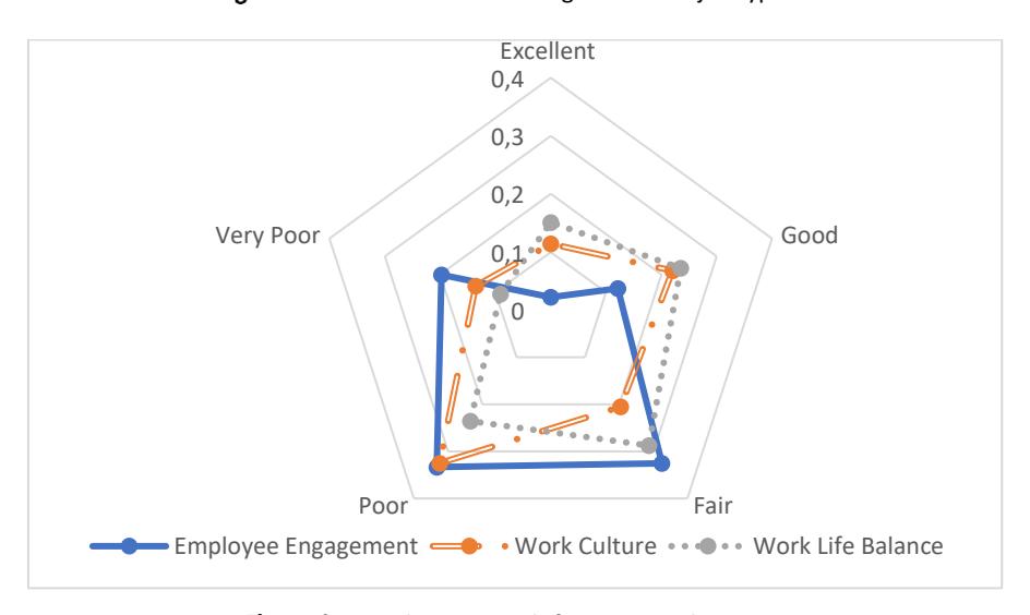
Evaluation result for private job type.
Figure 1 illustrates the outcome of a specific government job type and the components that comprise it. Employee engagement had risen toward the IV (Poor) level in the government sector, while work culture and work-life balance were shifting toward the III (Fair) level. Figure 2 displays the output of the private job type along with its components. In the private job type, employee engagement and work culture were inclined to IV (Poor) level along with work-life balance inclined to III (Fair) level. Overall, the findings indicate that in the private sector, job satisfaction is II (poor).
Workers in the public sector typically earn more than their private sector counterparts. (Reilly, 2013). This is because, in addition to competitive wages, public sector positions typically provide more extensive benefit packages, including health insurance, retirement plans, paid vacation, paid sick leave, and job stability.
Discussion
In summary, employers can improve job satisfaction by focusing on fair pay, creating a positive work culture, supporting work-life balance, prioritizing employee health and well-being, providing basic needs, ensuring job security, and supporting employees' families. Fair and Supportive Workplace: Employees want to know that their work is respected and that they are being paid enough for it. Employers can do this by giving fair pay, putting job stability first, and investing in the growth and training of their workers. A positive work culture that values teamwork, respect, and open communication can produce a supportive and collaborative environment that makes employees happy (Eisenberger et al., 2001). Work-life Balance and Well-being: Work-life balance is important for employees' health and happiness at work. Employers can set up policies like flexible work hours, paid time off, the option to work from home, access to mental health tools, wellness programs, and other health-related benefits to help people find a good balance between work and life (Susanto et al., 2022). Basic needs like clean water to drink, healthy food choices, and a safe, comfortable place to sleep should also be met. Family-friendly Policies: Employers can show they care about their workers' families by giving them benefits like paid family leave, help with childcare, and other family-friendly policies. Giving employees' children access to health and education tools can also be a good way to improve their health and happiness at work (Bae & Yang, 2017).
Implication of study
To enhance job satisfaction among civil engineers in Bagmati Province's transportation sector, employers should invest in employee development, offer competitive compensation, foster a supportive work environment, prioritize employee engagement, evaluate and improve policies, and implement family-friendly policies. Specifically, the low levels of job satisfaction observed, particularly among private sector employees, emphasize the urgent need for reforms in work culture, work-life balance, and employee engagement practices. These implications aim to create a more fulfilling and satisfying workplace, leading to increased productivity, reduced turnover, and overall improvements in the transportation infrastructure.
Likewise, this study's innovative methodological approach combines Mixed Set Questionnaire (MSQ), Principal Component Analysis (PCA), Structural Equation Modeling (SEM), and Multi-Dimensional Mapping (MDM) to comprehensively analyze job satisfaction. By using all of these approaches together, the study effectively deals with data collection, dimensionality reduction, relationship modeling, and response uncertainty. This technique makes job satisfaction analysis more thorough and reliable in business settings.
Conclusions
The research indicates that civil engineers employed in the transportation sector of Bagmati Province, Nepal, have a low level of job satisfaction Job satisfaction parameters like work culture, work-life balance, and employee engagement directly influence the employee's job performance. The survey revealed that civil engineers in the private sector experience low job satisfaction, whereas those in the government sector have moderate job satisfaction. Lastly, to improve job satisfaction among civil engineers in Bagmati Province's transportation sector, employers should implement a holistic approach encompassing employee development, competitive compensation, supportive work environments, enhanced engagement practices, and family-friendly policies, while future research should utilize the innovative PCA-SEM-MDM methodology to validate and refine these strategies across diverse contexts.
Acknowledgement
Researcher are deeply indebted to the Society of Transport Engineers Nepal (SoTEN), Er. Hemant Tiwari and Er. Anmol Thapa for providing access to valuable resources and data, which significantly contributed to the success of this study.
Compliance with ethics guidelines
The authors declare they have no conflict of interest or financial conflicts to disclose.
This article contains no studies with human or animal subjects performed by authors.