
Introduction
CNG as Fuel
In recent years, the increase in global population and urbanization has led to a significant increase in demand for oil, gas and iron ore consumption. Concurrently, the expansion of the economy and technological progress have played an important role in forcing developing countries to increase their needs for energy and metal resources. Increased investment in the discovery of oil, gas and mining is being actively encouraged to meet the estimated future demand in many countries. Subsequently, increased production activities, industry expansion and rising investments resulted in an increased requirement for high-capacity generators. These generators are indispensable in oil, gas and mining areas, where they play a required role in heavy-duty operations such as drilling and excavation. In nations where there is
1Research Scholar, Symbiosis Institute of Technology (SIT), Pune Campus, Symbiosis International (Deemed University) (SIU), Pashan-Sus Road, Pune, 412115, Maharashtra, India 2The Automotive Research Association of India (ARAI), Vetal Hill, Off-Paud Road, Pune 411038, Maharashtra, India.
Symbiosis Institute of Technology (SIT), Pune Campus, Symbiosis International (Deemed University) (SIU), Pashan-Sus Road, Pune, 412115, Maharashtra, India
4Technovuus, ARAI, Vetal Hill, Off-Paud Road, Pune 411038, Maharashtra, India
San Jose State University, San Jose, California, United States of America
frequent power scarcity, generators play an important role as they provide a reliable backup power supply. Increasing urbanization worldwide has increased the requirement for a consistent and reliable power source, resulting in the worldwide demand for generators (Fact.MR, 2024).
Compressed natural gas, or CNG, is now being used as a fuel choice for generators in cities and nearby areas. People rely on it because it offers cleaner energy that works better. CNG burns cleaner than diesel or petrol. Availability through pipeline systems also lessens the hassle of fuel storage and transportation. Generators powered by natural gas release fewer emissions and perform better with heat conversion. This makes them ideal in places with strict environmental rules or as backup power in critical locations like hospitals or office buildings (Prasad Rao & Karthikeya Sharma, 2020).
The Central Pollution Control Board (CPCB), which operates under the Ministry of Environment, Forest and Climate Change (MoEF&CC), sets emission rules for generator sets using CPCB standards. The new CPCB Stage IV+ norms now demand stricter goals requiring a 90% cut in NOₓ and particulate matter emissions when compared to those outlined in the CPCB Stage II standards. These rules push for changes in generator technology, such as adding electronic fuel injection, exhaust gas recirculation, and modern after-treatment systems (Mustafi & Agarwal, 2019).
Natural gas, which is methane, stands out among fuels due to its strong anti-knock properties. These properties allow spark ignition engines to work at higher compression ratios, increasing their overall efficiency. When compared to gasoline and diesel, engines running on compressed natural gas (CNG) produce fewer emissions of carbon monoxide, nitrogen oxides, and unburned hydrocarbons (Lather & Das, 2019). But CNG burns and has limited flammability, which can cause incomplete combustion or misfires under some conditions. This sometimes releases unburnt methane, a greenhouse gas that reduces some of its low-carbon benefits (Singh et al., 2016). The properties of CNG and Hydrogen as a fuel are given in Table 1.
To address these challenges, experts suggest using HCNG as a mixed fuel option. HCNG makes combustion better by speeding up the flame, shortening the ignition delay, and extending the lean burn range. This leads to steadier and fuller combustion, which lowers CO and HC emissions. Adding hydrogen also supports a steady shift toward using hydrogen in internal combustion engines while still working with existing fuel systems (Mustafi & Agarwal, 2019; Pathak et al., 2024). Studies show that HCNG cuts both regulated and unregulated emissions more than regular CNG during realworld operations like those specified in the ISO 8178 protocol (Singh et al., 2016). Using HCNG in generators shows potential to meet future emission standards while keeping performance reliable.
| Property | CNG | Hydrogen |
|---|---|---|
| LHV (MJ/kg) | 45.3 | 120.1 |
| Burning velocity in NTP air (cm/s) * | 45 | 325 |
| Flame speed (m/s) * | 0.37 | 1.7 |
| Density at NTP (kg/m3 ) | 0.668 | 0.0837 |
| Calorific value (MJ/kg) | 48.35 | 150 |
| Adiabatic Flame Temperature in air (K) | 2148 | 2318 |
| Auto ignition temperature (K) | 813 | 858 |
| Equivalence ratio | 0.7-4 | 0.1-7.1 |
Table 1 Summary of physical parameters.
Mixing hydrogen with CNG to produce HCNG helps in cutting down carbonyl emissions like formaldehyde and acetaldehyde. Hydrogen boosts combustion by increasing flame speeds, lowering ignition delay, and broadening flammability limits. Together, these changes lead to more thorough oxidation inside the engine cylinder (Zareei et al., 2020). Carbonyl compounds form during partial oxidation of hydrocarbons under fuel-rich or ignited conditions in CNG. Including hydrogen aids in generating more radicals such as H+ and OH-, which speed up oxidation reactions and reduce the time intermediate compounds stay in the process, curbing carbonyl emissions (Gong et al., 2016). Using HCNG also leads to higher temperatures and shorter burn times inside the engine, cutting back on incomplete combustion pathways. This has been shown in research to lower aldehyde emissions in engines running on HCNG when compared to those using standard CNG. This demonstrates how hydrogen supports cleaner and smoother combustion systems.
* - Laminar flame speed and burning velocity value are measured in standard conditions: environment pressure (1 ATM), initial temperature ~ 298 K, and using dry air as oxidizer. Reported flame speeds are the approximate values to suit the near-stoichiometric conditions (equivalence ratio ≈ 1.0).
Blending Hydrogen and CNG
Adding hydrogen to fuel mixtures creates notable effects. Hydrogen burns seven times faster than methane. This faster burning speed could improve combustion properties by shortening combustion times and boosting constant volume efficiency. Mixing hydrogen with natural gas enables leaner mixtures to reduce emissions (Park et al., 2011). HCNG, meaning hydrogen-enriched compressed natural gas, emerges as a promising option to replace traditional fossil fuels, cutting pollutants and enhancing engine performance. HCNG use could lead to sizeable drops in hydrocarbon and carbon monoxide emissions and might lower NOx emissions if the spark timing is optimized. This makes HCNG a strong candidate to provide cleaner energy choices for automotive uses (Choi et al., 2011).
Methane burns with a laminar flame speed eight times slower than hydrogen. Blending even a small amount of hydrogen with CNG shortens combustion times. Studies have measured how fast flames move in mixes of air, hydrogen, and methane at varying hydrogen levels and equivalence ratios. Results show that adding even a little hydrogen boosts combustion efficiency and cuts down on harmful emissions. This makes HCNG an option worth considering to produce cleaner energy (Ishaq & Dincer, 2020).
Adding hydrogen to CNG increases the fuel's quenching distance and lowers its carbon-to-hydrogen ratio. This change leads to more complete combustion while also cutting down HC and CO emissions. Hydrogen also expands the flammability range of CNG and makes lean combustion better. It helps reduce NOx emissions as well. Combining hydrogen with CNG speeds up the production of OH and H+ radicals. These radicals boost the combustion rate of CNG by enhancing reaction rates (Sofianopoulos et al., 2016). Using hydrogen in this way, the study aims to examine how HCNG compares to CNG in effectiveness.
Using a hydrogen-natural gas mix as fuel comes with some big challenges. Picking the right balance of hydrogen and natural gas is one of the hardest parts. If the hydrogen level goes beyond a safe point, and the air-fuel ratio or spark timing isn't set correctly, weird combustion can happen. Things like pre-ignition, knocking, or even backfiring may occur. To tackle these issues well, adjusting the air-fuel ratio and spark timing becomes crucial. This fine-tuning helps get the most out of HCNG while also reducing the risks that come with abnormal combustion.
Literature Review
Hydrogen-enriched compressed natural gas, often called HCNG, draws significant attention as a cleaner option to replace traditional fuels. It has the ability to improve how fuel burns and cut down on emissions containing carbon. Research demonstrates that adding more hydrogen to CNG blends boosts the efficiency of combustion. It does this by increasing in-cylinder pressure, how fast heat gets released, and how quickly the pressure builds. One example includes findings by Pandey et al. They recorded lower levels of CO, CO₂, and HC emissions and noted better brake thermal efficiency when the hydrogen content was higher. However, they also noted that NOₓ emissions tend to increase with hydrogen enrichment, though this effect is mitigated under high excess air ratios (Pandey et al., 2022).
Hydrogen addition is particularly effective under lean-burn and low-load conditions, as demonstrated by De Simio et al., who tested HCNG blends in light-duty and heavy-duty engines. They found combustion improvements to be more significant at low speeds and loads, although the overall engine efficiency gains were marginal under stoichiometric conditions (De Simio et al., 2011). Similarly, Hora and Agarwal documented that higher hydrogen concentrations (10– 30%) improved BTE, brake-specific fuel consumption (BSFC), and combustion behaviour, especially at higher loads, with a trade-off in increased NOₓ emissions. Enhanced performance was attributed to better combustion stability, elevated peak cylinder pressures, and improved cumulative heat release (CHR) (Hora & Agarwal, 2016).
In terms of thermal efficiency and energy density, several studies have evaluated the effects of stoichiometric and lean combustion regimes. Park et al. demonstrated that increasing hydrogen content up to 40% improved thermal efficiency and reduced CO and CO₂ emissions without affecting total hydrocarbons (THC). They also found that retarded spark timing yielded better emissions control than MBT ignition under HCNG operation (Park et al., 2011). Liu et al. further confirmed that thermal efficiency increases with hydrogen energy content, especially at lower engine loads, although NOₓ emissions rise correspondingly (Liu et al., 2017). On the contrary, Michikawauchi et al. reported that stoichiometric conditions reduced energy density and cruising range, although lean burn conditions using 50% hydrogen resulted in a 12% thermal efficiency gain compared to stoichiometric methane (Michikawauchi et al., 2011).
The lean-burn capability and stability of HCNG blends were further explored by Deng et al., who found that increasing hydrogen content from 0% to 75% improved indicated thermal efficiency, reduced cycle-to-cycle variations, and expanded the lean-burn limit. They highlighted that ignition timing optimization is critical to balance efficiency and emissions (Deng et al., 2011). Verma et al. studied blends ranging from 0% to 100% hydrogen to analyze their properties. They found that blends with an H/C ratio of 4.5 performed best in terms of heat efficiency. However, using pure hydrogen resulted in less efficiency because it has a lower energy density by volume (Verma et al., 2016).
Using machine learning (ML) algorithms alongside experimental research has helped predict combustion characteristics, cut down experiment time, and improve accuracy. Random Forest (RF) models show strong ability to capture complex nonlinear patterns in combustion data. Yang, Yan, Sijia, et al. compared ML models like RF and Artificial Neural Networks (ANN) to predict emissions such as CO, UHC, and NOₓ. They found both models work well, but RF models stand out with their reliability and easier interpretation (Yang, Yan, Sijia, et al., 2022). In another study, Papaioannou et al. applied RF models to predict particulate number, concentration, and geometric standard deviation in gasoline direct injection engines. Their findings highlighted engine power and blowby as key factors through permutation importance (Papaioannou et al., 2021).
Artificial Neural Networks, or ANNs, work well in handling multi-output modelling. Research by Yang, Yan, Sun et al. created an ANN model that gave accurate predictions for power, combustion timing like CA50, and emissions such as CO, UHC, and NOₓ. Their model reached R² scores higher than 0.97 (Yang, Yan, Sun, et al., 2022). Mehra et al. took a similar approach with an ANN model focused on a turbocharged HCNG engine. This model predicted torque, BSFC, and different emission levels with strong accuracy and minimal error using inputs like air ratio, engine load, and fuel mix (Mehra et al., 2018).
Support Vector Machines (SVMs) hold potential when dealing with small datasets and intricate patterns. Hao et al. applied SVMs to make predictions about torque, BSFC, and NOₓ in HCNG engines. Their results showed that SVMs achieved accurate predictions by modelling how the excess air ratio and ignition timing affect performance (Hao et al., 2020).
Alongside standard models, researchers have used hybrid and ensemble methods to study fuel-blend performance. Sonawane et al. applied the TOPSIS approach to estimate key performance factors like power, torque, and combustion time in ethanol-gasoline mixtures. Their results showed R² values above 0.95 and MAPE ranging from 1% to 5%, pointing to strong potential for accurate calibration (Sonawane et al., 2023). In a similar exploration, Airamadan et al. evaluated combustion stability and fuel use in spark-assisted gasoline compression ignition engines by comparing models like CatBoost linear regression, SVM, and RF. Leave-one-out cross-validation confirmed the generalization capabilities of these models across varying operational regimes (Airamadan et al., 2022).
In summary, literature underscores the dual advantage of HCNG as a low-emission, high-efficiency fuel and machine learning as a critical enabler for predictive combustion modelling. Hydrogen enrichment enhances combustion quality, particularly under lean conditions, while ML models such as RF, ANN, SVM, and hybrid approaches offer high-accuracy prediction tools for emissions and performance. When coupled with hyperparameter optimization strategies like GridSearchCV, these models can significantly reduce experimental requirements, support calibration strategies, and accelerate the deployment of cleaner internal combustion technologies.
Even with progress in HCNG engine modelling and predictive combustion tools, key research challenges remain. Most machine learning studies stick to single-cylinder engines or rely on simulated setups, offering little validation on multicylinder engines that mirror how engines perform in real-world settings (Sahoo et al., 2022). Research also overlooks how we can scale performance data from low hydrogen blends to high ones. This method could make experiments less time-consuming (Farhan et al., 2024). Most predictive tools either concentrate on emissions or performance, but fail to combine crucial combustion factors like Pmax, IMEP, and combustion duration into a single model (Duan et al., 2023). Optimization of models, through methods such as GridSearchCV, is also underused in Random Forest or Artificial Neural Network-based approaches (Rao et al., 2023).
To tackle these issues, this study tests different HCNG blends on a multi-cylinder engine running at a constant speed. It uses a high-resolution data acquisition tool for more precise measurement. A Random Forest regression model helps predict combustion behaviour and engine performance. Data from lower blends is used to estimate the behaviour of higher blends. Hyperparameter tuning refines the model to improve prediction accuracy and reduce overfitting. By tying together both combustion and performance predictions under one system and validating it through real-world experiments, this work takes a step toward creating more efficient, reliable, and scalable HCNG engine models.
Methodology
The methodology for engine testing, experimentation, and selecting the appropriate machine learning model for this study is provided in the following sections.
Experimentation
The study was done on a water-cooled, naturally aspirated, inline, 6-cylinder SI engine, equipped with a three-way catalytic converter as an after-treatment system. This engine has a wedge-type combustion chamber, which is typically used in SI engines. Specifications of the test engine are given in Table 2. This engine was connected to a SAJ make, 150kW capacity, and an eddy current dynamometer using a cardan shaft. CNG and various HCNG blends were used as test fuels. The air-fuel mixture was inducted into the intake manifold through the throttle body. The real-time fuel mass flow rate was acquired by installing a Coriolis mass flow meter (Emerson, CMF010M).
| Displacement | 6.59 L |
|---|---|
| Aspiration | Naturally Aspirated |
| Engine Type | Inline, Single Speed |
| Compression Ratio | 17.5:1 |
| Polytropic Coefficient | 1.37 |
| Rated Power | 55 kW |
| Rated Speed | 1500 RPM |
Table 2 Engine Specifications.
The assessment followed a 3-mode test cycle (D2) for a constant-speed engine, as outlined in ISO 8178-4 and shown in Figure 1. The manufacturer-specified rated power and rated speed of the engine can be utilized to compute the maximum load (in Nm) to be applied to the engine. The engine is tested at 100%, 75%, and 50% of the rated torque. The list of equipment used for the experimentation is given in Table 3.
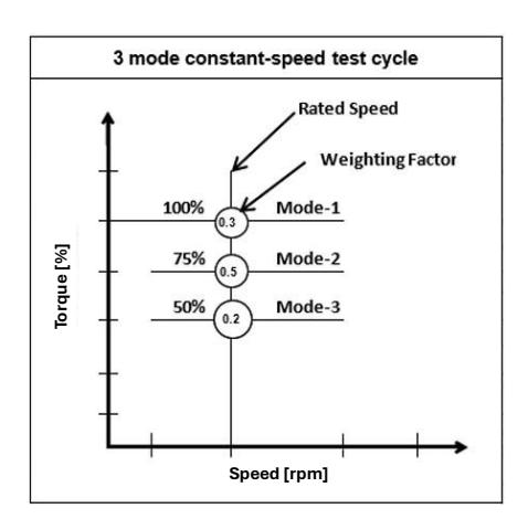
ISO 8178 D-2 Test Cycle.
Table 3 List of Equipment used for experimentation.
| Dyno make | SAJ AG 150 |
|---|---|
| Air Flow meter | ABB Sensiflow SFI-11 |
| Air Conditioning Unit | KS CAHU |
| Raw Emission Measurement System | AVL AMA i60 |
| Fuel Flow Meter | Emerson, CMF010M |
| Combustion Pressure Sensor | AVL GH12D |
| HSDA system | AVL Indimicro |
The engine is first warmed up so that the oil temperature is above 65℃. The engine is then set at 100% load condition using the T% mode of the engine dyno. The emission data and other engine performance parameters are recorded once the engine achieves stability for the set point. This point is called Mode 1 of the test cycle. Similarly, the other two modes of the test cycle are set, and the data is acquired.
The intake air is carefully maintained at optimal atmospheric conditions (25°C and 45% relative humidity) by the Conditioned Air Handling Unit (CAHU). It then passes through an air filter, which acts as a barrier between the ambient air - laden with particulate matter - and the sensitive interior of the engine. Subsequently, the air enters the intake manifold, where it interfaces with the fuel injected at a pressure of 2 bar in the combustion chamber. The HCNG blends were stored at a pressure of 200 bar in a cylinder cascade, and the fuel was passed through a pressure reduction unit before entering the engine. Throughout the test cycle, the air-fuel mixture was maintained stoichiometrically. Additionally, pressure and temperature sensors are strategically placed on various parts of the engine to measure the steady-state engine conditions.
In this experimental study, in order to minimize the impact of cyclic fluctuations, the combustion data was collected for 300 consecutive cycles and the average dataset was used for further analysis. We obtained in-cylinder pressure data using an AVL make piezoelectric pressure sensor (GH12D), which comprised a pressure transducer capable of measuring dynamic pressures up to 250 bar, a charged amplifier, and a measurement cable. The charge produced by the pressure transducer was converted into a proportional voltage signal using a charged amplifier, and this signal was then captured by the high-speed combustion data acquisition (HSDA) system.
In this experimental study, the effects of cyclic variations during combustion were reduced by collecting combustion data over 300 consecutive cycles and then using the average data for further analysis. For measuring in-cylinder pressure, an AVL piezoelectric pressure sensor (model GH12D) was used, which included a pressure transducer capable of recording dynamic pressures up to 250 bar, along with a charge amplifier and a measurement cable. The charge generated by the pressure transducer was transformed into a corresponding voltage signal through the charge amplifier, and this signal was subsequently recorded by the high-speed combustion data acquisition (HSDA) system.
The crankshaft was acquired with a crank angle encoder that serves as a reference for measuring the crank angle and is utilized for analyzing engine combustion. The collected data is plotted against the crank angle to calculate various thermodynamic parameters. A schematic of the experimental setup with the data acquisition system is given in Figure 2. The HSDA data was acquired from a variety of sensors, and the combustion curves, including heat release rate, cumulative heat release rate, and combustion temperature, were derived from the in-cylinder pressure curve. Furthermore, parameters such as the start and end of combustion, combustion duration, and IMEP were also determined for both CNG and HCNG blends.
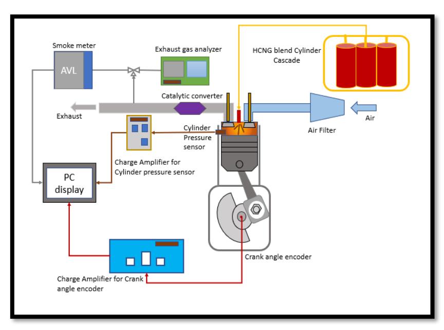
Experimental Setup with HSDA system for Combustion analysis.
The calculation model was developed in the AVL Concerto software, which is used to read the acquired data files from the AVL system and represent the data graphically as a function of crank angle. The engine was initially tested on compressed natural gas (CNG), and then, gradually, various blends of hydrogen-enriched compressed natural gas (HCNG) were tested using the same engine calibration as CNG. This was intentionally carried out to evaluate the performance and emission differences when using different fuels with the same engine calibration in order to determine the calibration adjustments needed to optimize the engine parameters for the fuel blend. Engine performance, combustion, and emission data for CNG and HCNG blends containing 18% Hydrogen (18HCNG) and 25% hydrogen (25HCNG) were collected. Figure 3 shows the comparison of the combustion data collected for CNG and 18HCNG.
From Figures 3 and 4, it can be inferred that the addition of hydrogen reduces the combustion duration by almost 10% from CNG to 18HCNG. This is because the Mass Burnt Fraction of 90% (MBF90) is achieved faster, owing to the higher flame speed of hydrogen than that of CNG, which is 1.7 m/s for Hydrogen as compared to 0.4 m/s for CNG fuel. Similarly, the Heat Release Rate (HRR) for 18HCNG is higher than the HRR for CNG. This is due to the higher calorific value of Hydrogen (150 MJ/kg) as compared to CNG (48.35 MJ/kg). This means that the Hydrogen molecule releases more energy than the Methane (CH4) molecule when it is ignited.
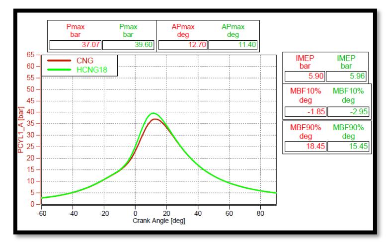
Pressure vs Crank angle for CNG vs 18HCNG.
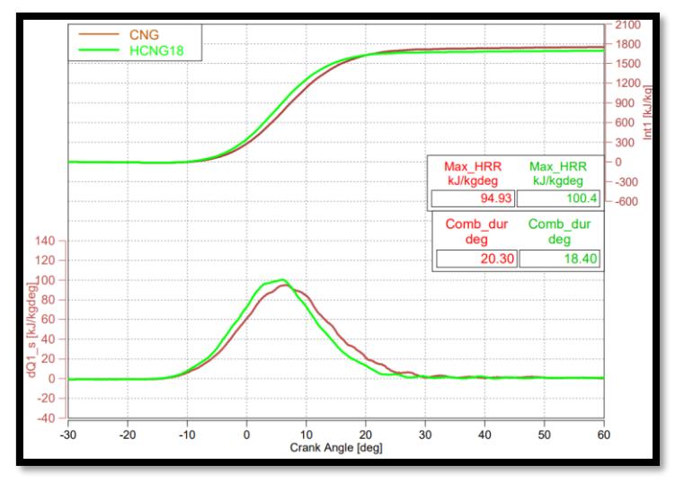
Heat Release Rate curves for CNG and 18HCNG.
The maximum cylinder pressure of 18HCNG is higher than that of CNG due to spontaneous combustion and the rapid rise of cylinder pressure because of the spontaneous combustion of Hydrogen in the 18HCNG fuel blend. This is also reflected in the crank angle duration at which the maximum pressure is attained (APmax). The APmax for 18HCNG achieved is 11.40°CA, which is around 10.23% faster than that of CNG fuel.
The peak temperature for 18HCNG (Figure 5) has decreased as the engine operates in a lean condition. This results in a lower peak combustion temperature due to the deviation from the stoichiometric air/fuel ratio. Consequently, lean combustion leads to lower peak temperatures, providing an advantage for reducing NOx emissions in 18HCNG. Overall, blending CNG with Hydrogen has shown improvement in combustion characteristics.
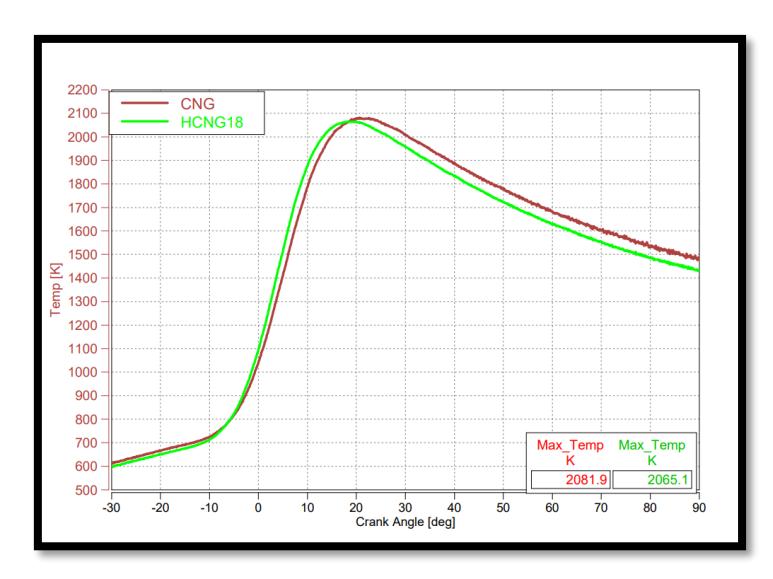
Temperature curves for CNG and 18HCNG.
To gather emissions data, we used a raw exhaust gas emission analyzer (AVL AMA i60) to measure NO, HC, CO, CO2, and O2 concentrations in the engine exhaust. The sample comparison of emissions (in ppm) for the CNG and 18HCNG blend is illustrated in Figure 6.
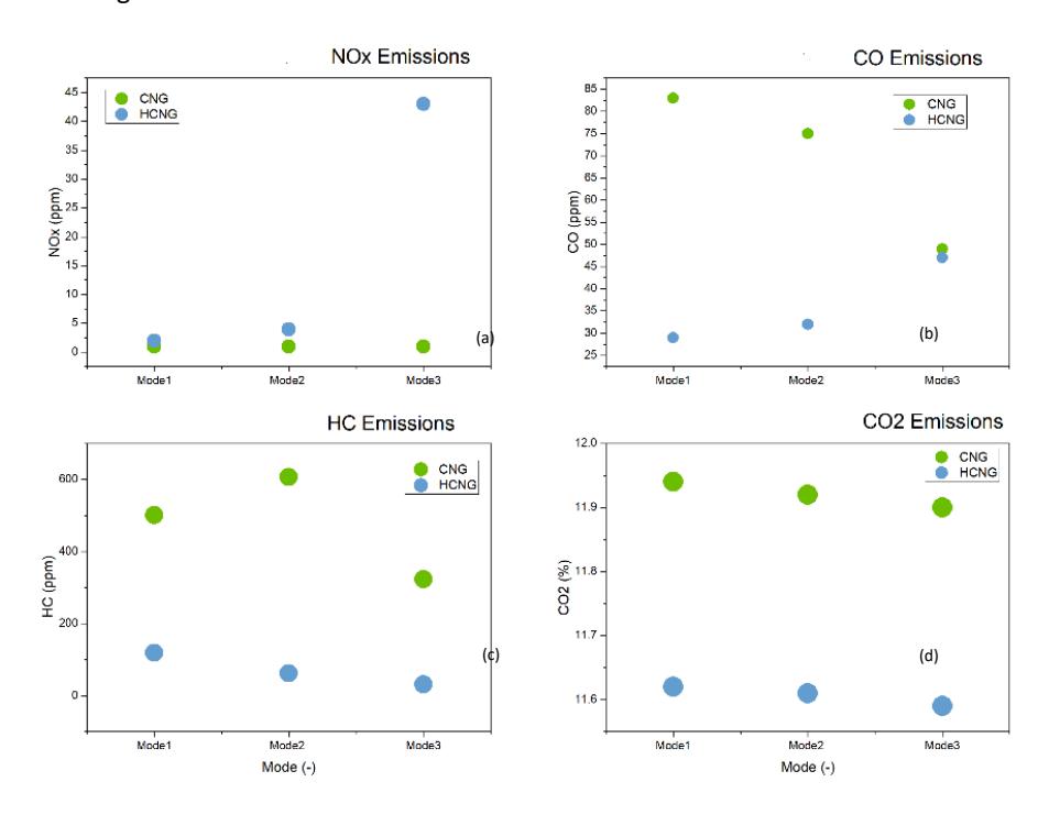
Comparison of NOx, HC, CO and CO2 emissions for CNG and 18HCNG.
The NOx emissions for 18HCNG have increased across all 3 modes compared to CNG due to higher combustion temperatures. However, HC emissions have decreased by 85%, and CO emissions have been reduced by 56% for 18HCNG. This reduction is attributed to the lower H/C ratio in the HCNG blend, which leads to more complete combustion at higher temperatures, thereby lowering CO and HC emissions.
Although the temperature profile (Figure 5) indicates a marginal reduction in peak combustion temperature for the 18% HCNG blend compared to pure CNG, primarily due to leaner operation and deviation from the stoichiometric air–fuel ratio. The NOx emissions were observed to increase across all three modes of the CPCB emission cycle as per ISO 8178. This apparent contradiction is explained by the complex interplay between flame speed, combustion phasing, and localized thermal behaviour introduced by hydrogen enrichment. The presence of hydrogen enhances flame propagation and reduces ignition delay, resulting in earlier combustion phasing and a sharper rise in temperature closer to top dead centre (TDC). This shift increases the residence time of combustion gases within the critical temperature window for NOx formation, even if the absolute peak temperature is slightly lower. Moreover, at intermediate and partload conditions during the 3 modes, the combined effects of moderate equivalence ratios and faster combustion lead to elevated local temperatures and prolonged high-temperature residence, both of which are conducive to increased thermal NOx production. Hence, the rise in NOx emissions with HCNG operation is not solely governed by global peak temperature but by the broader thermodynamic and kinetic changes induced across the engine cycle.
Machine Learning
Machine learning (ML) plays a significant role in establishing connections between engine responses and control variables, thereby facilitating global search optimization based on specific merit functions and enabling easier sensitivity analysis. Thanks to these advantages, the ML algorithm has been successfully and widely used in predicting various engine-related parameters, including power, pressure, phasing, exhaust gas temperature, engine vibrations, emissions, efficiency, and fuel composition effects.
Here is a comparison of the performance and combustion data of CNG and lower blends of HCNG 18% and HCNG 25% to predict the performance and combustion characteristics of the higher blend of HCNG 30%. After that, these predictions were compared with experimental data. Two models for the purpose of this work were developed: one for performance characteristics and the other for combustion characteristics. As for the regression algorithm, it was chosen after a detailed analysis of different factors and previous models implemented in prediction in the literature review.
Choosing a Machine Learning Model
In the research literature on predicting engine performance using machine learning techniques, the most commonly used algorithms were Random Forest and Artificial Neural Network (ANN) (Yang, Yan, Sijia, et al., 2022), (Papaioannou et al., 2021), (Sonawane et al., 2023), (Mehra et al., 2018), (Airamadan et al., 2022), (Yang, Yan, Sun, et al., 2022), (Shah et al., 2019). Some papers also mentioned the use of a Support Vector Machine (SVM) for predicting BSFC and NOx emissions (Hao et al., 2020).
The Random Forest algorithm was chosen for developing the model over Artificial Neural Networks (ANN) because of the following points:
- 1. The Random Forest (RF) algorithm is a more cost-effective option that doesn't necessitate a GPU for training and can achieve satisfactory results with fewer data points. It offers an alternative interpretation of decision trees while delivering improved performance. In contrast, Neural Networks typically require a significantly larger dataset than what an average user may possess to function effectively.
- 2. The RF algorithm has one more advantage in that it applies a greedy algorithm during training, as described in the Methodology section. This helps Random Forests to determine the important parameters for the model as there is no need for other independent algorithms to assess the parameter importance (Papaioannou et al., 2021). A neural network can increase the complexity of the model to improve performance, but at the expense of the interpretability of features. If comprehension of the variables is crucial, then some performance may have to be sacrificed for the model to clearly display how each variable impacts the prediction.
The Random Forest is an ensemble approach used in machine learning for regression as well as classification tasks. In this approach, multiple decision trees are used and a technique known as Bootstrap and Aggregation or bagging is used. The basic concept is that instead of using one decision tree to get the result, the final result is obtained by combining the results of multiple decision trees. The base learners in Random Forest are multiple decision trees. The sample datasets for each model are created by randomly sampling the rows and features of the dataset and this is referred to as Bootstrap.
The Random Forest algorithm consists of a collection of decision trees and can be applied to classification as well as regression tasks. The final output is determined by averaging the results from all the individual decision trees. In this model, the variables being predicted include engine torque, fuel flow rate, and exhaust gas temperature. This method effectively captures complex relationships among the variables for accurate predictions. It is widely used in various engineering applications for performance analysis.
discussed in greater detail in subsequent sections of this study.
The decision tree partitions the parameter space into branches by applying a threshold that changes with each split, as represented in the first line of each box in Figure 7. The parameters and thresholds for these splits are chosen based on a specific performance criterion, such as squared error, which is also depicted in Figure 7. The tree continues to split until it reaches a terminal node (leaf), where a single prediction is made, as shown by the value in Figure 7. Furthermore, the splitting process and the number of terminal nodes can be managed through various hyperparameters, which are
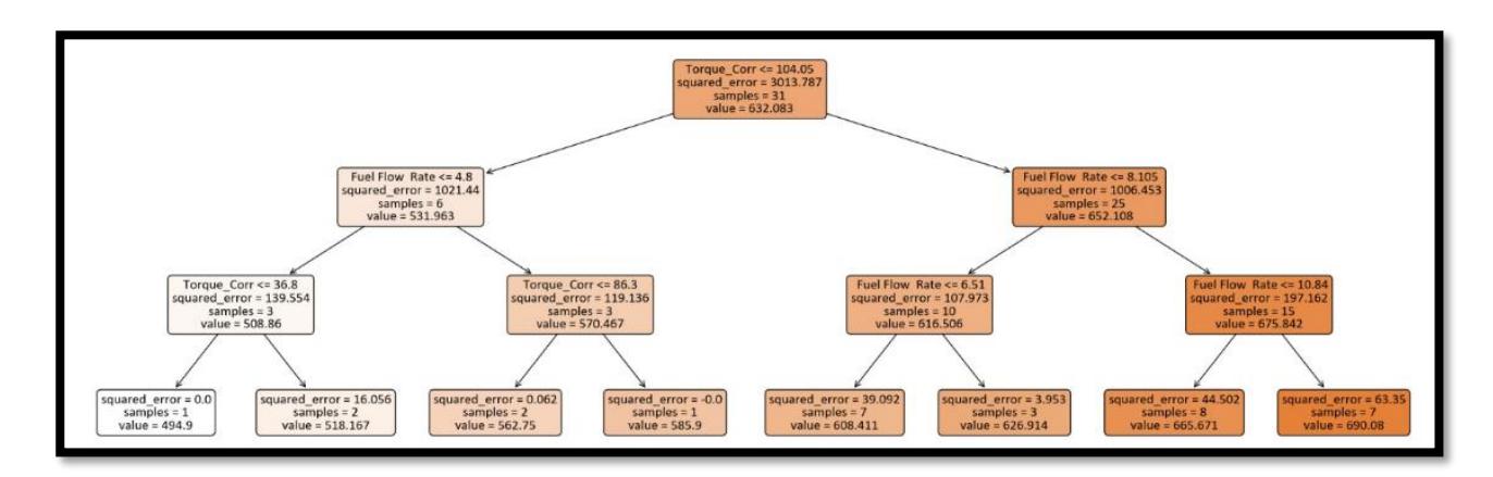
A Random Forest Decision tree for Performance data prediction.
Once the tree is fully developed (meaning the model has been trained), each partition will represent a specific subset of the target variable, and the model's output for that partition will be the average of this subset. A larger tree creates more partitions, which can enhance the model's accuracy and detail. Random Forests compute the average output of the various decision trees through a technique called bagging. For each individual tree, sampling is often done using bootstrapping, which involves sampling with replacement. This method results in trees that are inherently diverse.
In the decision trees, every sample parameter and data point is considered when forming each node. This can lead to overfitting, where the model becomes overly fitted to the training data and fails to generalize well to new data, especially as the size of the dataset increases. A slight change in the data can produce a completely different tree structure. This is where Random Forests become advantageous, as they help reduce the risk of overfitting by averaging the results of multiple trees.
Machine Learning Results
This section presents the machine learning results for performance and combustion parameters for the multi-cylinder engine with HCNG blends investigated in the present work.
Random Forest Modelling for Engine Performance Parameters
A Random Forest regression model was trained on the experimental data of 18HCNG and 25HCNG, which included the input and output parameters as mentioned in Error! Reference source not found..
| Input Parameters | Output Parameters |
|---|---|
| Fuel intrinsic property | |
| (Calorific value/ Laminar Burning speed) | Exhaust Temperature |
| Torque | BMEP |
| Fuel flow rate | BSFC |
| Air/Fuel ratio |
Table 4 Input and Output parameters for the Performance RF model.
The experimental data available for the parameters in question included only 10 data points for each blend. Given that there are three blends (with 18% and 25% used for training and 30% for validation), this results in a total of just 30 data points for training, which is inadequate for effectively training a machine learning model. To address this limitation, the practice of synthetic data generation is commonly employed across various industries. This approach helps create more robust models and fosters improvements in performance. In the context of the big data era, synthetic data generation
holds significant promise, particularly for supporting advancements in the Internet of Things (IoT). It plays a crucial role in realizing concepts such as digital twins and cyber-physical systems on a broader scale.
The use of synthetic data is picking up momentum in engineering when it comes to modelling systems that are both complex and nonlinear. Collecting large amounts of real-world data for such tasks can sometimes be too expensive or not possible. Sonawane et al. showed how adding synthetic data through nonlinear interpolation improved predictions in gasoline-ethanol engine performance using Random Forest models (Sonawane et al., 2023). Ghareeb et al. took a similar approach with vehicle seat thermal dynamics, showing its real-world value in managing automotive heat systems (Ghareeb et al., 2024). The effectiveness of these techniques has been demonstrated in the simulation of electronic package behaviors (Lee & Kwon, 2025), while Kou et al. focused on diagnosing faults in mechanical components (Kou et al., 2019). Hou et al. explored its role in predicting electric vehicle battery wear and tear (Hou et al., 2021). Studies confirm that these techniques keep the original dataset's nonlinear patterns intact and help models perform better with ensemble methods like Random Forest (Cheng et al., 2024; Kim et al., 2024). Altogether, these examples show how nonlinear interpolation-based synthetic data can be a reliable and useful tool in engineering-related machine learning studies.
A non-linear interpolation method was implemented to create additional synthetic data, resulting in an expansion of the 30 experimental runs to 500 data points. This enhancement aimed to improve the precision of model training and the accuracy of predictions while simultaneously reducing overall testing costs and time.
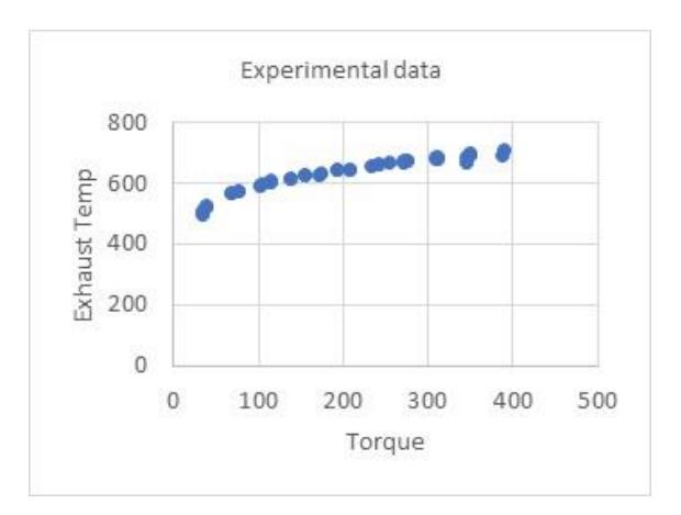
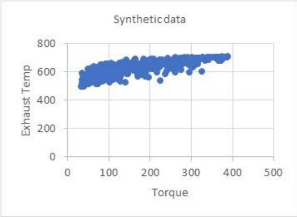
Synthetic data generation from Experimental data points for Exhaust Temperature.
The data includes Experimental and Synthetic data for 18% and 25% HCNG blends for the output parameter of Exhaust temperature, as shown in Figure 8. Similarly, synthetic data for BMEP and BSFC were generated. The model was trained on 80% of the data and tested on 20% of the data. A regression model was created using Random Forest regression on the experimental and synthetic data for 18HCNG and 25HCNG blends. The RF model summary for engine performance parameters is given in Table 5.
| Exhaust Temperature | BSFC | BMEP | |
|---|---|---|---|
| R2 | 95.88% | 94.26% | 92.99% |
| RMSE | 10.00 | 35.64 | 0.67 |
| MAPE | 1.34% | 9.18% | 19.26% |
Table 5 RF Model Summary for Engine Performance Parameters
To ensure that the synthetic data generated via non-linear interpolation accurately reflects the distributional characteristics of the original experimental dataset, a statistical validation procedure was conducted. Specifically, goodness-of-fit tests were applied to all input features to evaluate the similarity between the real and synthetic data distributions. For numerical features, the two-sample Kolmogorov–Smirnov (K–S) test was employed, while Pearson's chi-squared test (χ²) was reserved for categorical variables, where applicable. The K–S test checks how the empirical cumulative distribution functions of the two samples compare. In this case, it examines 30 experimental points against 500 synthetic ones to spot any major statistical differences. Researchers used Python (v3.10) with the
'scipy.stats.ks_2samp' function to analyze the data, setting a significance level (α) of 0.05. The test showed no major statistical deviations between the experimental and synthetic data distributions across all tested features. This finding verifies that the interpolated dataset aligns well with the original data structure. Because of this, the synthetic dataset represents the real data. This reduces the chance of bias, underfitting, or overfitting when training models. Figure 9 shows a statistical validation of the synthetic BSFC data distribution as a sample.
The Kernel Density Estimation (KDE) plot compares the distribution of BSFC between experimental and synthetic datasets. The curves are nearly overlapping, indicating high similarity. Whereas the Empirical Cumulative Distribution Function (ECDF) comparison, with a K–S test p-value, displays that the p-value is well above 0.05, there is no significant difference between the distributions, confirming that the synthetic data reliably mimics the experimental data.
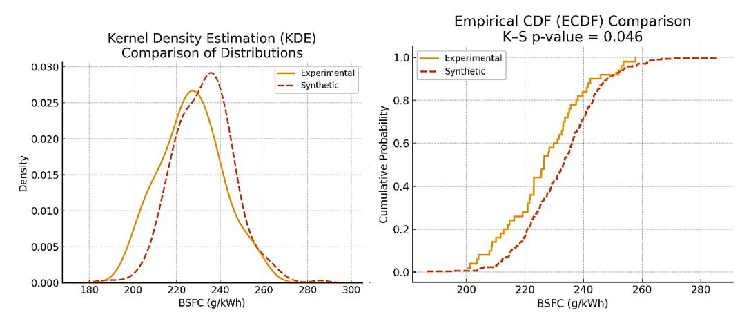
Statistical Validation of Synthetic Data Distribution Using KDE and ECDF for BSFC.
Evaluating Model Robustness: Performance Assessment in the Absence of Synthetic Data
The Random Forest model demonstrated high predictive accuracy when trained on the non-linear interpolated dataset comprising 500 samples. Performance metrics such as R² scores exceeding 92%, low RMSE, and MAPE values across engine performance parameters (Exhaust Temperature, BSFC, BMEP) indicate that the model captured the underlying trends and relationships effectively within the expanded data space. However, to assess the true generalizability of the model, a comparative experiment was conducted by training and testing the Random Forest model using only the original 30 experimental data points.
| Table 6 | RF model summary for experimental data points without synthetic data. |
|---|
| Exhaust Temperature | BSFC | BMEP | |
|---|---|---|---|
| R2 | 82.6% | 79.4% | 72.3% |
| RMSE | 17.8 | 54.6 | 1.04 |
| MAPE | 6.45% | 16.88% | 28.74% |
Table 6 shows the RF model output for experimental datapoints without the synthetic data. As expected, the model's performance declined noticeably under the constrained data regime compared to its performance with the synthetically augmented data regime (Table 5). The R² values dropped to 82.6% for Exhaust Temperature, 79.4% for BSFC, and 72.3% for BMEP, representing a 10–20% reduction in explanatory power. Similarly, the RMSE values increased to 17.8, 54.6, and 1.04, respectively, while MAPE rose sharply to 6.45%, 16.88%, and 28.74%. These results reflect the onset of overfitting, where the model, limited by the small dataset, tends to memorize localized data patterns rather than learning generalizable trends. The steep rise in MAPE, particularly for BMEP, also indicates increased sensitivity to input noise and poor extrapolation ability. This performance gap underscores the importance of synthetic data in compensating for experimental limitations and justifies the use of methods like non-linear interpolation to enhance training diversity and improve model robustness.
Effect of Interpolated Synthetic Data on Model Generalization and Overfitting
To investigate the influence of data volume and distribution on model performance, the Random Forest regression model was trained separately on two datasets: one comprising only the original experimental data (30 samples), and the other augmented to 500 samples using a non-linear interpolation method. When trained solely on experimental
data, the model exhibited clear signs of overfitting, as evidenced by high training R² values (0.98 for BMEP, 0.97 for exhaust temperature, and 0.94 for BSFC), but significantly lower test R² values (0.77, 0.68, and 0.27, respectively) as shown in Figure 10. The substantial drop in performance, especially for BSFC, indicates that the model learned localized patterns specific to the training set but failed to generalize beyond them, typical of high-variance behaviour associated with small datasets.
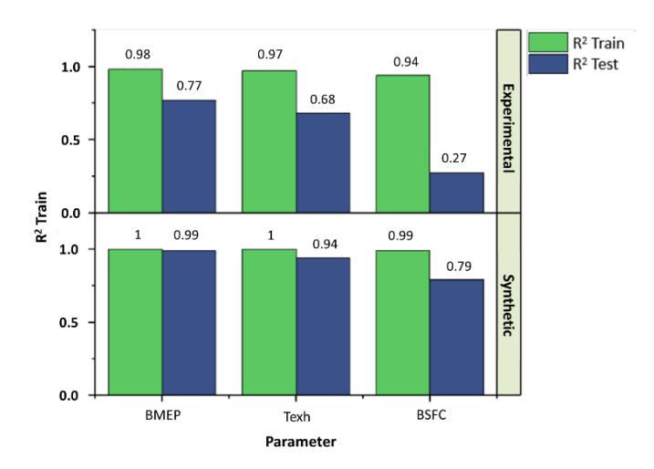
Comparative R² Scores for RF Model Trained on Experimental vs Synthetic Datasets.
In contrast, the model trained on the interpolation-augmented dataset showed marked improvement in generalization, with test R² values rising to 0.99 for BMEP, 0.94 for exhaust temperature, and 0.79 for BSFC. The relatively small difference between training and testing performance suggests that interpolated synthetic data helped to smooth transitions in the feature space and reinforce functional relationships between input variables. However, it is important to recognize that non-linear interpolation introduces deterministic data that may lack the natural noise and variability of experimental conditions. This can result in subtle biases, especially in parameters like BSFC, where real-world fluctuations are more pronounced. The slight reduction in generalization accuracy for BSFC (compared to BMEP) likely reflects this limitation. Therefore, while non-linear interpolation is a practical and computationally efficient approach to expand training datasets, care must be taken to ensure that interpolated points do not misrepresent complex realworld behaviours, particularly in sensitive combustion metrics.
Random Forest Modelling for Combustion Parameters
The HSDA data was generated for three different modes of a single-speed multi-cylinder engine (at 100%, 75%, and 50% of the rated torque) for CNG, 18HCNG, and 25HCNG. The input and output parameters of the model are listed in Tbale 7.
| Table 7 | Input and Output parameters for Combustion RF model. |
|---|---|
| Input Parameters | Output Parameters |
|---|---|
| Blend (% H2) | Maximum Combustion Pressure |
| Fuel Intrinsic Property (Calorific value/ Laminar Burning speed) | IMEP |
| Torque | Combustion duration |
The HSDA data was used to obtain various combustion characteristics over 300 cycles. Due to the raw nature of the data, 50 cycles of data were selected for each mode, as the variation in characteristics was not very uniform over the entire 300 cycles. Specifically, data for 18% and 25% HCNG blends at 100%, 75%, and 50% of the rated load was chosen to create a machine-learning model using the Random Forest Regression method mentioned in the previous section. An 80:20 train-test split was used as it was found to produce better results based on trial-and-error observations.
A regression model was created using Random Forest regression on the experimental data for 18HCNG and 25HCNG blends. The model summary for engine combustion parameters is given in Table 8.
Table 8 RF model summary for engine combustion parameters.
| Pmax | IMEP | Comb_dur | |
|---|---|---|---|
| R2 | 95.17% | 99.82% | 92.99% |
| RMSE | 2.17 | 0.06 | 0.39 |
| MAPE | 3.99% | 0.73% | 1.41% |
The Random Forest model shows strong performance across all three metrics for Pmax, IMEP, and Combustion Duration (Comb_dur), with IMEP having the best fit and smallest error margins, indicating that the model is highly effective, especially in predicting IMEP. The model has slightly higher errors for combustion duration as compared to IMEP.
From the model summary data shown in Table 5 and Table 8 it is evident that the model has a higher error in predicting BSFC, BMEP and Combustion Duration. In order to have the predictions for the 30HCNG fuel blend, the model needs to be more accurate. Hence, it was decided to optimize the Random Forest Regression model.
Optimization of Regression Model
Random Forest (RF) involves several hyperparameters that dictate the structure of each individual tree, as given in Table 9. These hyperparameters include the minimum node size required for a node to be split, the number of trees in the forest, and the degree of randomness in the model. Additionally, Random Forest considers the number of variables deemed as candidate splitting variables at each split, as well as the sampling scheme used to generate the datasets on which the trees are built.
Table 9 Hyperparameters in Random Forest Regression.
| Hyperparameter | Description | Typical Default Values |
|---|---|---|
| mtry | Count of candidate variables selected for each split | √p, p/3 for regression |
| samp_size | Count of observations being drawn from each tree | n |
| replace | Observations being drawn with or without replacement | TRUE (with replacement) |
| min_node_size | The terminal node containing a minimum number of observations | 1 for classification, 5 for regression |
| max_depth | Each decision tree's maximum depth | |
| n_estimators | Number of trees contained in the forest | 500, 100 |
| split_rule | Splitting criteria of the nodes | Gini impurity, p-value, random |
| min_samples_split | The minimum number of samples required to split an internal node | 1 |
In machine learning, tuning involves finding the best hyperparameters for a given dataset and learning algorithms. In supervised learning, such as regression and classification, optimality can be defined in terms of different performance measures like error rate or AUC, as well as the runtime, which can be influenced by hyperparameters in certain cases.
To optimize the performance of the machine learning model, GridSearchCV was implemented, which applies the Grid Search technique to find the best hyperparameters. With GridSearchCV, a range of values is defined for the selected parameters, and then every combination of these parameters is iterated thoroughly to identify the combination that improves the chosen cost function the most.
Table 10 displays the optimal hyperparameters found using GridSearchCV for predicting the outputs of the engine performance and combustion parameters. These hyperparameters include the number of estimators, maximum depth, and the minimum number of samples needed to split an internal node. Once these best hyperparameters are known, they are used to optimize the Random Forest regression model. This helps to lower the errors and enhance the accuracy of the model.
Table 10 Selection of the best hyperparameters for all the RF model outputs.
| Hyper parameters | Values of parameters given in the grid | Exhaust Temp | ВМЕР | BSFC | Pmax | IMEP | Combustion Duration |
|---|---|---|---|---|---|---|---|
| max_depth | 10, 20, 30, 40, 50 | 30 | 20 | 50 | 30 | 10 | 10 |
| min_samples_split | 5, 10, 15, 20 | 20 | 20 | 10 | 20 | 5 | 15 |
| n_estimators | 100, 200, 300, 400, 500 | 100 | 300 | 100 | 100 | 100 | 200 |
The Random Forest regression model was then run to predict engine performance parameters for 30HCNG data. The model summary is given in Table 11.
| Table 11 RF Model Summary for Engine Performance Parameters after Optimization for 30HCNG Blend. |
|---|
| Exhaust Temperature | BSFC | BMEP | |
|---|---|---|---|
| R2 | 96.77% | 97.69% | 98.63% |
| RMSE | 7.95 | 12.29 | 0.26 |
| MAPE | 1.27% | 3.93% | 5.43% |
The optimized Random Forest model shows strong performance across all parameters, with particularly high precision for BMEP in terms of R² and RMSE, with very accurate predictions with low percentage errors for exhaust temperature. The optimized model has improved the MAPE for BMEP and BSFC from 19.26% to 5.43% and from 9.18% to 3.93%, respectively. This indicates the model is a highly accurate fit but with a slightly higher percentage error (>5%), possibly due to the nature of BMEP's scale or the specifics of the data used.
The hyperparameters for the combustion data prediction model were optimized as per Table 8. Then, the model was run to predict engine combustion parameters for 30HCNG data. The model summary is given Table 12.
Table 12 RF Model Summary for Engine Combustion Parameters after Optimization for 30HCNG Blend.
| Pmax | IMEP | Comb_dur | ||
|---|---|---|---|---|
| R2 | 96.24% | 99.85% | 95.50% | |
| RMSE | 1.93 | 0.06 | 0.30 | |
| MAPE | 2.48% | 0.64% | 1.11% | |
The optimized Random Forest model shows excellent performance across all measured parameters, with good predictive power and moderate errors relative to the scale for maximum combustion pressure (Pmax). The model has exceptionally high accuracy with very low errors both in absolute and percentage terms for IMEP predictions for 30HCNG. Whereas, for combustion duration, the model gives a strong performance with slightly higher errors compared to IMEP but is still very accurate. The optimized model has improved the R2 for Combustion Duration from 92.99% to 95.50%, which has a more than 95% confidence level to predict the combustion duration for the 30HCNG blend.
Discussions
The outputs obtained from the optimized Random Forest regression model were validated with experimental data using a 30% HCNG blend. The RF model outputs for the engine performance and combustion parameters are discussed against actual experimental values for the 30HCNG blend in the subsequent sections.
Assessing the Predictive Strength of Random Forest Relative to Other Machine Learning Algorithms
In the literature, various machine learning models have been employed to predict engine performance and combustion characteristics, including Artificial Neural Networks (ANN), Support Vector Machines (SVM), Gradient Boosting methods, and Random Forests (RF). ANN models, as demonstrated by Mehra et al. and Yang et al., are capable of modelling complex nonlinearities but suffer from interpretability issues and require extensive hyperparameter tuning and large datasets for stable performance (Mehra et al., 2018; Yang, Yan, Sun, et al., 2022). SVMs, utilized by Hao et al., offer good generalization in smaller datasets but are highly sensitive to kernel selection and lack built-in mechanisms to evaluate feature importance (Hou et al., 2021). Gradient Boosting algorithms such as CatBoost and XGBoost, explored by Airamadan et al., provide slightly improved accuracy over RF in some cases but come with higher computational costs and are more susceptible to overfitting, especially in noisy or synthetic datasets (Airamadan et al., 2022). In contrast, the Random Forest method used in this study provides a strong trade-off between accuracy, interpretability, robustness to noise, and minimal tuning. Particularly in data-constrained environments augmented with generative methods like CTGAN, RF shows consistent generalization while preserving transparency in decision-making through feature importance analysis. The comparative assessment of the ML algorithms based on the above-mentioned literature survey for engine performance modelling is given in Table 13.
| Model | Handling of Nonlinearity | Performance on Small Datasets | Feature Importance Interpretation | Sensitivity to Synthetic Data Quality | Training Complexity | Overfitting Risk |
|---|---|---|---|---|---|---|
| Random Forest (RF) | Excellent | High | Yes (Built-in via feature importance) | Low to Moderate | Low | Low |
| Artificial Neural Network (ANN) | Excellent | Poor without augmentation | No (Black box) | High | High | High |
| Support Vector Machine (SVM) | Good | Moderate | No | Moderate | Moderate | Moderate |
| Gradient Boosting (e.g., CatBoost, XGBoost) | Excellent | Moderate | Partial (with SHAP tools) | High | High | High |
| TOPSIS/ MCDM Methods | Not applicable | Not applicable | Yes (Ranking- based) | Not applicable | Very Low | Not applicable |
Table 13 Comparative Assessment of Machine Learning Algorithms for Engine Performance Modelling.
Engine Performance Data Analysis
To assess the predictive capabilities of the Random Forest regression model, a comparison between actual and predicted values was carried out for the 30% HCNG blend under the ISO 8178 D2 3-mode cycle. As depicted in Figure 11, the model demonstrates a close agreement between the actual and predicted exhaust temperatures across the torque range, highlighting its strong predictive capability in capturing thermal behavior trends.
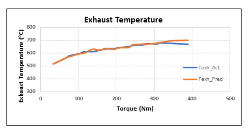
Figure 11 Exhaust Temperature Actual vs Predicted values.
Similarly, Figure 12 illustrates the brake-specific fuel consumption (BSFC), where the predicted values closely follow the actual curve, particularly in the high-torque range, underscoring the model's ability to learn non-linear fuel efficiency characteristics. The BSFC prediction curve exhibits noticeable deviation from the actual experimental data at lower torque values, particularly below 100 Nm. This mismatch suggests that the Random Forest model, despite its overall high predictive accuracy, struggles to generalize accurately in the low-torque regime. This behavior is primarily attributed to error bias introduced during model training, especially when the data distribution in the low-torque region is sparse or exhibits high variability.
Hence, the model's performance degradation at low torques in BSFC prediction can be directly linked to training data imbalance and inherent limitations in learning finer combustion dynamics in low-load conditions. This underscores the necessity of ensuring a more uniformly distributed and representative training dataset, potentially through synthetic data augmentation, to improve model generalization across the full torque range.
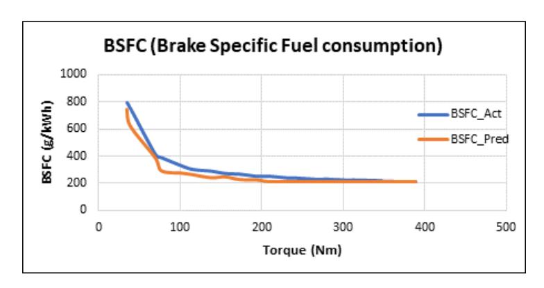
BSFC Actual vs Predicted values
The comparison for Brake Mean Effective Pressure (BMEP), shown in Figure 13, further supports the model's robustness, as the predicted BMEP trajectory is nearly indistinguishable from the actual measurements. Collectively, these three figures confirm the high fidelity of the Random Forest model in replicating engine performance characteristics based on a 30HCNG blend.
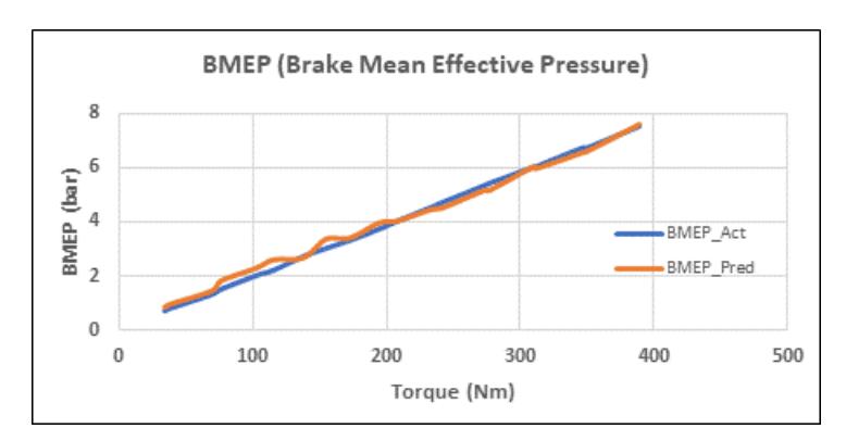
BMEP Actual vs Predicted values.
From the graphs shown above, the Random Forest regression model is highly precise in predicting the engine performance parameters for the 30HCNG blend. The engine was tested with 30% HCNG as per the ISO 8178, D2 3-mode test cycle. The comparative data w.r.t various HCNG fuel blends and CNG is discussed based on engine performance parameters like brake thermal efficiency (BTE), BSFC, and BMEP. Beyond the model predictions, engine performance across varying HCNG blend ratios is presented in the subsequent section.
Figure 14 shows the BTE at 3 modes for the HCNG blends. The BTE for 30HCNG is slightly lower as compared to the 25HCNG blend. When hydrogen is added to compressed natural gas, and the engine speed is increased, the brake thermal efficiency (BTE) typically decreases. In the case of our single-speed engine, where the engine speed remains constant, the increase in calorific value outweighs the decrease in mass flow rate. As a result, for the same torque, the brake thermal efficiency decreases as the percentage of hydrogen in the blend increases. The BTE remains relatively stable in Mode 1 for all blends, but slightly decreases with increasing hydrogen concentration, particularly for 30HCNG in Modes 2 and 3. This reduction is attributed to the combined effects of fixed engine speed and changes in mass flow rate. Although hydrogen increases the calorific value of the blend, the overall energy conversion efficiency slightly declines due to alterations in combustion phasing at higher hydrogen percentages.
Figure 15 shows the BSFC of different HCNG blends at the 3 modes. The BSFC shows a decreasing trend with an increase in the hydrogen content. This is attributed to the higher energy content of the fuel blend as a result of the addition of hydrogen, which has a calorific value more than twice that of CNG. The higher hydrogen content contributes to improved fuel efficiency and performance, making HCNG blends an interesting area for further research and development in the field of alternative fuels. The inverse relation between hydrogen enrichment and BSFC underscores the potential of HCNG in optimizing fuel economy, especially in steady-state generator operations.
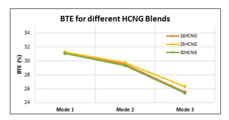
Mode-wise BTE (Brake Thermal Efficiency) for different HCNG blends.
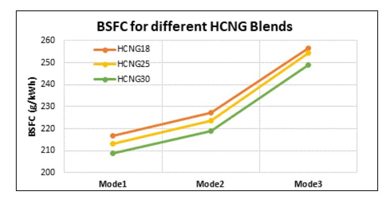
Mode-wise BSFC for different HCNG blends.
An analysis was conducted on the temperature trend of the exhaust gas after the manifold across three different modes. Figure 16 shows the exhaust temperature trend for various HCNG blends at 3 modes. It shows that the addition of hydrogen in the blend resulted in the highest exhaust gas temperature for 18HCNG. As the blend was transitioned to 25HCNG, the temperature of the exhaust gas began to decrease, reaching its lowest point for the 30HCNG blend.
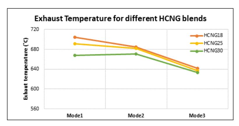
Mode-wise Exhaust temperatures for different HCNG blends.
When hydrogen is added to natural gas, the resulting increase in flame temperature leads to higher exhaust gas temperatures under both stoichiometric and fuel-lean operating conditions. This rise in flame temperatures enables more complete combustion. As the percentage of hydrogen in the mixture continues to increase, the exhaust temperature initially rises and then decreases due to spontaneous combustion.
Together, these observations affirm that the Random Forest model effectively captures engine performance trends for HCNG blends, while the comparative analysis of BTE, BSFC, and exhaust temperature substantiates the potential benefits and limitations of increasing hydrogen proportions in dual-fuel strategies.
Engine Combustion Data Analysis
The Random Forest regression model was validated using 30% HCNG blend data, and various evaluation measures were used to assess its accuracy and predictability. The average of predicted and actual values over 50 combustion cycles for a specific mode was compared, as the individual data did not follow a specific trend. The results of the comparison for the predicted and actual values of 30% HCNG blend for Pmax, are shown in Figure 17, whereas IMEP and Combustion Duration at the 3 modes are represented in Figure 18.
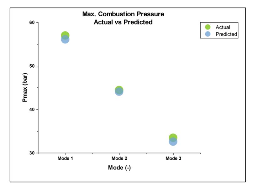
Maximum Pressure at 3 modes: Predicted vs Actual.
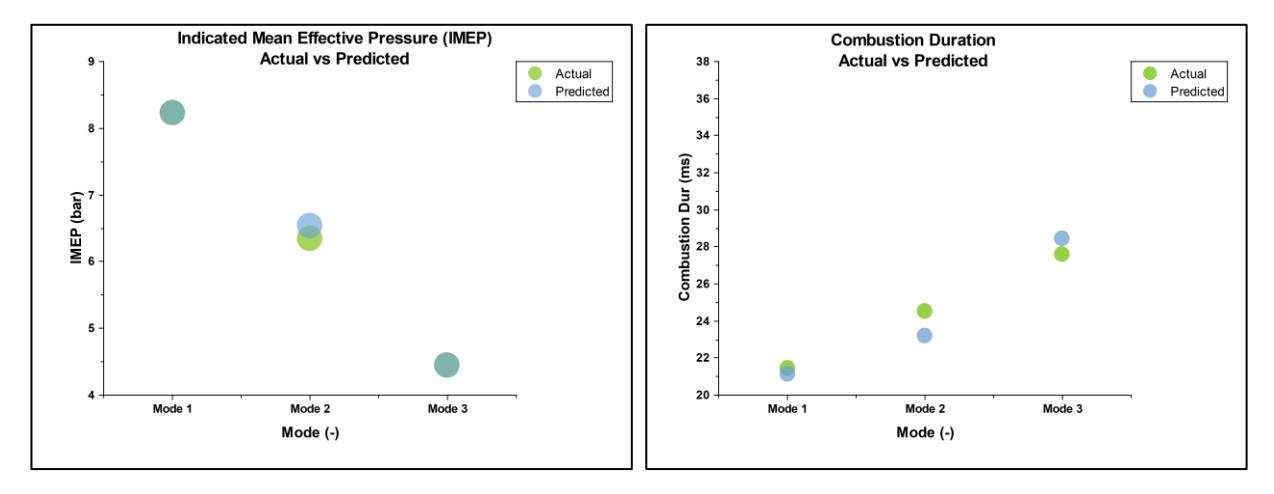
IMEP and Combustion at 3 modes: Predicted vs Actual.
The Random Forest regression model predicts Maximum pressure, IMEP, and Combustion duration with an error of less than 3%. This small error is due to the data being acquired over CNG calibration, and there is also cyclic variation in airfuel ratio as the engine attempts to correct the fuelling based on a closed-loop strategy.
As stated earlier, the engine was tested with 30% HCNG as per the ISO 8178, D2 3-mode test cycle. The comparative data w.r.t various HCNG fuel blends is discussed based on engine combustion parameters like maximum combustion pressure (Pmax), IMEP, and Combustion duration.
The combustion data for mode 1 is shown in Figure 19. For mode 1, the torque is maximum torque, and hence, there is very little difference in the peak combustion pressure (Pmax) values and therefore, the IMEP is also similar. The maximum combustion temperature is lower for higher hydrogen blends as the combustion occurs spontaneously within
less time as compared to lower hydrogen blends. The cumulative heat release rate (Int1) is also lower for 30HCNG as compared to 18HCNG.
The combustion data for mode 2 is shown in Figure 20. The experimental findings indicate a 4% increase in combustion pressure and temperature when the hydrogen blend increases from 18% to 30%. This rise in pressure and temperature is primarily due to the accelerated burning rate within the fuel-air mixture, along with a decrease in the mixture's heat capacity. Also, the occurrence of the peak pressure (APmax) is shifted towards the TDC side (near 0 crank angle) from 11.4CA to 10.6CA. This shows that the combustion duration is reduced by 7.5% as the hydrogen blend is increased from 18% to 30% at mode 2.
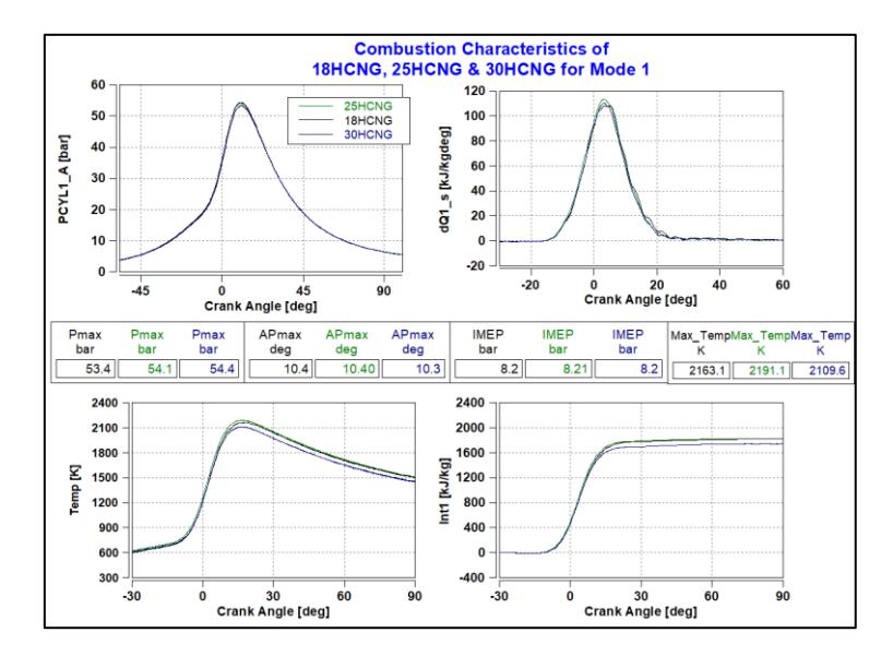
Combustion Characteristics for various HCNG blends at Mode 1.
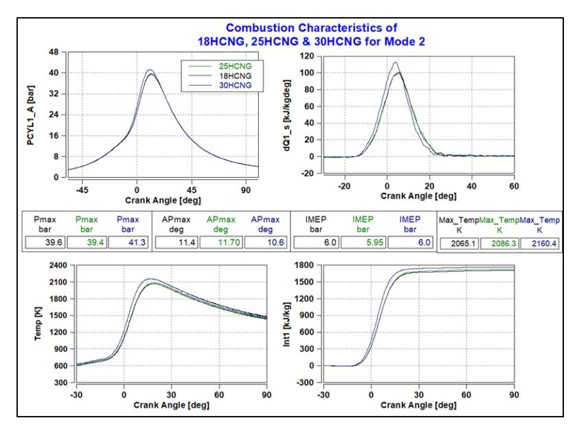
Combustion Characteristics for various HCNG blends at Mode 2.
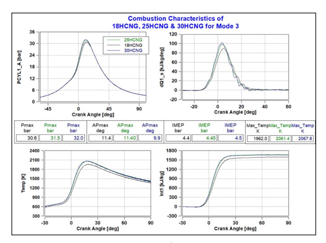
The combustion data for mode 3 is shown in Figure 21. The experimental findings indicate around 5% increase in combustion pressure and temperature when the hydrogen blend increases from 18% to 30%. Also, the occurrence of the peak pressure (APmax) is shifted towards the TDC side (near 0 crank angle) from 11.4CA to 9.9CA. This shows that the combustion duration is reduced by 15% as the hydrogen blend increases from 18% to 30%. This observation suggests a correlation between the hydrogen content and the timing of maximum heat release, indicating that the combustion process accelerates with increased hydrogen content in the blend. This effect can be attributed to the high flame speed of hydrogen, which enhances the combustion process and contributes to shorter combustion durations in the HCNG blends.
Combustion Characteristics for various HCNG blends at Mode 3.
Emissions Analysis
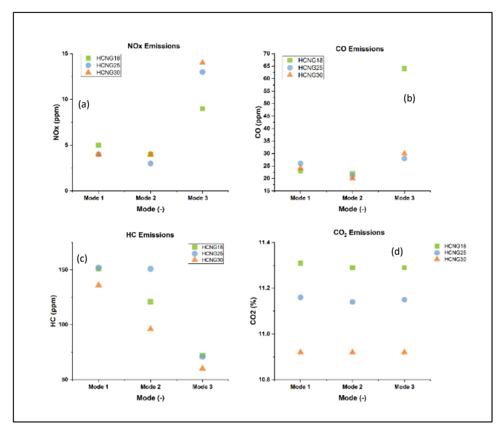
The engine underwent initial testing using natural gas and was calibrated accordingly. Subsequently, the same calibration was utilised for testing HCNG blends with varying hydrogen concentrations of 18%, 25%, and 30%. The emissions obtained for HCNG blends cannot be compared directly for raw emission calculation because of the different exhaust gas densities. Bandyopadhyay D. et al. described that the ratio between densities of gas components and exhaust gas, called μgas, is different for different fuel blends and is an exclusive value that changes as per the fuel composition (Bandyopadhyay et al., 2025). Here, the authors normalize or correct emissions across different HCNG blends using a method based on unit mass of fuel burned, leveraging exhaust gas density (μgas) and exhaust volume flow rates. This approach allows for fair and consistent comparison of emissions across blends with different hydrogen fractions. The raw emission concentrations (in ppm or %) are converted into mass flow rates (e.g., g/s) by multiplying with the exhaust gas density (μgas) and the exhaust flow rate. This avoids errors that arise from comparing just concentration values when flow rates differ between blends. Accordingly, the emission results were gathered for each blend across three operational modes, and the comparative analysis is visually depicted through graphs showcasing the emission values in Figure 22.
The use of an 18HCNG blend results in a notable decrease in NOx emissions, with this reduction becoming more pronounced as the proportion of hydrogen in the blend increases. This phenomenon is attributed to the decrease in residual time of the combustion mixture in the combustion chamber as the hydrogen ratio rises, resulting in a subsequent decrease in chemical NOx. Additionally, there is a substantial reduction of 62% in HC emissions and 85% in CO emissions when utilizing 18HCNG compared to CNG. Moreover, these emissions show a further decline for 25HCNG and 30HCNG. This significant reduction is linked to the increase in combustion temperature, which promotes more thorough combustion.
Variations in NOx, HC, CO and CO2 emissions for 18HCNG, 25HCNG and 30HCNG.
Conclusion and Future Scope
This study utilized a Random Forests algorithm to accurately predict performance parameters like BMEP, BSFC, Exhaust temperature, and combustion parameters such as maximum pressure, IMEP, and combustion duration for lower blends (18% and 25%) of HCNG on a Genset engine across various operating conditions.
To improve the prediction accuracy, the 'GridSearchCV' was used to test the performance of different combinations of parameters to determine the best model hyperparameters and the optimal combination was selected. Additionally, highly correlated parameters were eliminated prior to model training to enhance the performance of the permutation importance algorithm.
The optimized and trained model showed impressive accuracy across all target variables. Additionally, when validated with an independent dataset that was not part of the training process, the model performed exceptionally well even for a higher fuel blend. The prediction accuracy for engine performance parameters, especially for BMEP, the prediction accuracy improved by 6% to 98.63%. Also, for engine combustion parameters, the combustion duration prediction accuracy improved by 3% to 95.50%. Thus, improving the Mean Absolute Percentage Error (MAPE).
This outcome is notable as it indicates that a single model was able to accurately predict all three target variables. Such performance suggests that the model is not only robust but also capable of generalizing well to new data, which is a crucial aspect of effective machine-learning applications.
In the case of single-speed engines, the increased energy density of the fuel with increasing hydrogen content is more significant than the decrease in the mass flow rate of the fuel. This is because as the percentage of hydrogen increases in CNG, BTE is decreasing. There is also a very large decrease in BSFC hence an improvement in fuel efficiency with increasing hydrogen blending in CNG. This is mainly because the energy density of the fuel blend increases with increasing hydrogen content.
The combustion pressure and IMEP are increasing as a result of the increase in hydrogen percentage in the HCNG blend because hydrogen in the fuel blend burns faster. At the same time, the combustion period is also reduced for higher HCNG blends as compared to CNG and other lower HCNG blends.
The CO and NOx emissions at full loads have been reduced for higher HCNG blends as compared to CNG or lower HCNG blends because of the lower residence time of the air-fuel mixture in the combustion chamber which is beneficial for suppression of NOx emissions. As CNG is replaced by hydrogen fuel, carbon emissions are reduced. Hydrogen combustion occurs more rapidly compared to CNG combustion, resulting in lower CO emissions as the hydrogen percentage in the HCNG blend increases.
In Machine Learning, future work may involve using an ANN model for prediction when additional experimental data is available. Furthermore, comparing the Random Forest model's results with non-tree-based models like artificial neural networks, which would require more hyperparameter tuning and validating their predictions through actual engine experiments, could be considered.
More parameters like emissions of NOx, HC, and CO can be predicted by conducting several emission tests.
Compliance with ethics guidelines
The authors declare they have no conflict of interest or financial conflicts to disclose.
This article contains no studies with human or animal subjects performed by authors.