
Introduction
As the need for mineral resources continues to rise and the industry exhausts easily accessible reserves, the mining industry increasingly focuses on enhancing extraction and metal recovery methods. This has led to mining operations extending to greater depths beneath the Earth's surface (Lippmann-Pipke et al., 2011). From 2018 to 2021, global mineral consumption showed a relative upward trend (Our World in Data, 2023), indicating that the global demand for mineral resources will continue to grow. To meet this growing need, underground mining must probe deeper geological formations to find potential resources. As the depth of mines increases, the overburden pressure increases, resulting in higher stress levels within rock masses (Singh et al., 2010). This, in turn, increases the possibility of occupational accidents due to intensified environmental hazards (Xue et al., 2019).
Historically, between 1900 and 2022, more than 85,000 workers died due to mining accidents (Mine Safety and Health Administration, 2023). After the first recorded case in 1738 in Britain, rockbursts have become one of the most common underground mining accidents, especially in China (Xue et al., 2020). Between 1933 and 2018, China recorded more than 3,000 rockburst cases in 177 underground mines spread across more than 20 provinces in China (Wang et al, 2019). Meanwhile, from 1936 to 1993, the United States reported more than 172 cases of rockbursts, with more than 78 deaths (Ullah et al., 2022). Rockbursts are sudden and violent rock failures involving the ejection of rock fragments and rapid release of energy, typically associated with seismic events, and causing severe damage to underground structures (He et al., 2023). They are responsible for many mining accidents, damaged excavations, financial losses, and operational disruptions in the mining facilities (Adach-Pawelus & D. Pawelus, 2021).
Given the above context, the significance of identifying effective preventive measures cannot be overstated. By proactively addressing rockburst risks through research, innovation, and industry-wide adoption of safety protocols, the mining sector can not only protect the lives and well-being of its workforce but also safeguard its long-term viability by reducing the frequency of accidents and the substantial financial toll associated with these catastrophic events. Along with technological development, machine learning has emerged as an alternative solution to various realworld problems. It is often used in predicting and classifying problems in various fields, including engineering (James et al., 2013). In this respect, Wang et al. (2022), Ullah et al. (2022), and Zheng et al. (2023) used extreme gradient boosting (XGBoost) to classify the intensities of rockbursts. They demonstrated that XGBoost is a viable machine learning model given its great ability to classify rockburst intensities. Ullah et al. (2022) utilized XGBoost to classify rockburst intensities using 93 observations of rockburst cases and six features that affect rockbursts: cumulative number of events, event rate, log cumulative release energy, log energy rate, log cumulative apparent volume, and log apparent volume rate. The rockburst intensities were divided into four classes (none, slight, moderate, and intense). The proportion of the target classes was considered slightly imbalanced, with 36%, 23%, 27%, and 14% in the none, slight, moderate, and intense classes, respectively. There were four evaluation metrics: accuracy, precision, recall, and F1-score. Using tdistributed stochastic neighbor embedding and K-means clustering, XGBoost achieved 88% accuracy, 0.91 precision, 0.88 recall, and 0.88 F1-score.
Li et al. (2023) used eight types of support vector machines (SVMs) to classify coal burst intensity classes, 95 observations of coal burst case, and four features that affect coal bursts: dynamic failure time, elastic energy index, impact energy index, and uniaxial compressive strength. The intensities of coal bursts in this research were divided into three classes: none, weak, and strong. The proportion of the target classes was considered imbalanced, with 6.32%, 47.37%, and 46.32% in the none, weak, and strong classes, respectively. This previous work used three metrics: accuracy, F1-score, and kappa coefficient. Grey Wolf Optimization (GWO–SVM) emerged as the best model with 98.9% accuracy, an F1-score of 0.993, and a kappa coefficient of 0.98.
Other studies on rockburst intensity classification have been conducted using various machine learning models. For example, Wojtecki et al. (2021) using 150 rockburst observations, applied various algorithms, such as decision tree (DT), random forest, gradient boosting (GB), and artificial neural network, to evaluate rockbursts in the upper Silesian coal basin in Poland. Zhou et al. (2012) using 132 rockburst observations, classified long-term rockbursts by adopting the SVM model, and their results were recommended for underground rockburst assessment.
This paper classifies rockburst events in underground mines, along with their intensities using GWO–SVM and XGBoost. These rockburst events are classified as: existent and none, and their intensities are classified into four categories: none, weak, moderate, and strong. The data consists of 476 rockburst observations with six variables: maximum tangential stress, uniaxial compressive strength, uniaxial tensile strength, stress coefficient, rock brittleness coefficient, and elastic strain index. This study aims to support the mitigation of rockbursts in underground mining operations.
In Section 2, the data and methodology of this research are described as follows: rockburst classification, the data used, and the methods. Section 3 presents the classification results of rockburst events and their intensities for each model. In Section 4, we provide an in-depth analysis in the discussion. Finally, the conclusion is drawn in Section 5.
Data and Methodology
Data
Rockbust events are classified into two classes: (i) The Existent class refers to the presence of a rockburst event, regardless of its intensity. This class consists of three rockburst intensity classes: weak, moderate, and strong. (ii) The None class indicates the absence of rockburst events in underground mines. This class indicates a lack of significant fractures on the free face. Meanwhile, the weak rockburst class involves small specimens with minor fragment displacement and kinetic energy release. The moderate rockburst class shows deformations and fractures affecting the surrounding rocks and leading to the sudden release of a substantial amount of rock fragments. The strong rockburst class represents severe rock fractures, sudden ejections, powerful explosions, rumbling noises, persistent air blasts, and turbulent phenomena, with rapid expansion deep into the surrounding rock (He et al., 2023).
The dataset used in this study combined data from Zhou et al. (2012) and Xue et al. (2020), with 478 rockburst observations. As there were some missing values in the label column, which included three rockburst intensity classes (weak, moderate, and strong), data cleaning was performed. The final dataset consisted of 476 rockburst observations with imputed values for variables that affect rockburst intensity, including maximum tangential stress, uniaxial compressive strength, uniaxial tensile strength, stress coefficient, rock brittleness coefficient, and elastic strain index. Table 1 shows a sample of the dataset.
| Maximum Tangential Stress | Uniaxial Compressive Strength | Uniaxial Tensile Strength | Stress Coefficient | Rock Brittleness Coefficient | Elastic Strain Index | Intensity |
|---|---|---|---|---|---|---|
| 90.00 | 170.00 | 11.30 | 0.53 | 15.04 | 9.00 | Moderate |
| 90.00 | 220.00 | 7.40 | 0.41 | 29.73 | 7.30 | Weak |
| 62.60 | 165.00 | 9.40 | 0.38 | 17.53 | 9.00 | Weak |
| 55.40 | 176.00 | 7.30 | 0.32 | 24.11 | 9.30 | Moderate |
| 30.00 | 88.70 | 3.70 | 0.34 | 23.97 | 6.60 | Moderate |
Table 1 Sample of the dataset.
Maximum tangential stress occurs in an object or material when a load or force is applied, causing the material to distort. Uniaxial compressive strength is the ability of an object or material to withstand the pressure of an applied load or force parallel to its axial axis. Uniaxial tensile strength is the ability of an object or material to resist the pull of a load or force applied parallel to its axial axis. Meanwhile, the stress coefficient is the ratio between the maximum strength of a material and the force required to cause the material to fail or break. The rock brittleness coefficient is a numerical parameter used to measure the extent to which a rock is brittle or soft. Finally, the elastic strain index is a numerical parameter that measures the ability of a rock formation to withstand mechanical loads applied to the rock and produce elastic deformation. Figure 1 shows the distribution of various rockburst classes.
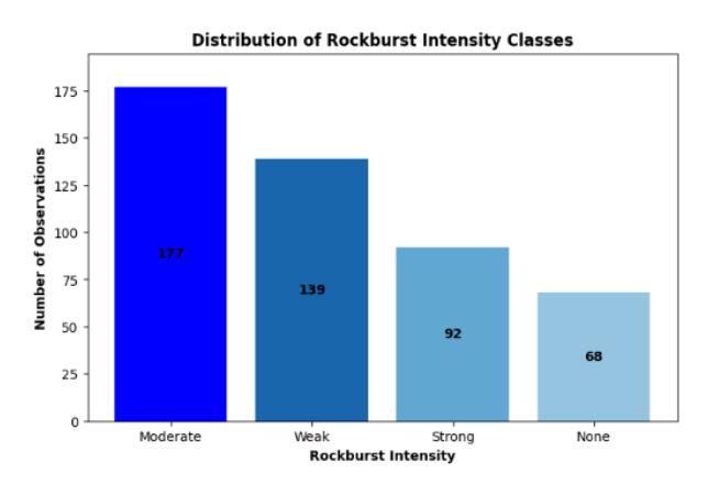
Distribution of rockburst intensity classes.
Most of the observations were in the moderate class with 177 observations (37.2%). The weak class had 139 observations (29.2%), the strong class had 92 observations (19.32%), and the none class had 68 observations (14.28%). Table 2 shows the statistical description for each feature of the dataset. As the range of values of the features used was diverse, the feature range was rescaled.
| Descriptive Statistic | Maximum Tangential Stress | Uniaxial Compressive Strength | Uniaxial Tensile Strength | Stress Coefficient | Rock Brittleness Coefficient | Elastic Strain Index |
|---|---|---|---|---|---|---|
| Mean | 48.159 | 114.862 | 6.519 | 0.444 | 20.669 | 4.307 |
| Std. Deviation | 24.181 | 43.014 | 3.320 | 0.215 | 8.929 | 2.096 |
| Minimum | 2.600 | 18.32 | 0.380 | 0.090 | 0.147 | 0.810 |
| Maximum | 114.440 | 235.000 | 17.200 | 1.100 | 47.930 | 10.900 |
Table 2 Statistical descriptions of the dataset.
Methodology
First, we classify the occurrence of rockbursts using GWO–SVM and XGBoost. This information is important for safety measures, regardless of the explosion's size. Second, we employ the same models to classify rockburst intensities. This information helps us mitigate the severity of rockbursts. In other words, this research enables the early detection of rockburst size or intensity using the prediction results. Figure 2 depicts the flow of this research.
This research starts with a literature review and data collection, followed by data preprocessing, including missing value handling through data cleaning, mean imputation, outlier checking using the interquartile range (IQR), and target class balancing in the training set using the synthetic minority oversampling technique (SMOTE). The two machine learning models are used to classify rockburst events before classifying their intensities. Finally, rockburst events in underground mines and their intensity classification were evaluated and compared in terms of accuracy, precision, recall, F1-score, and computation time using GWO–SVM and XGBoost models.
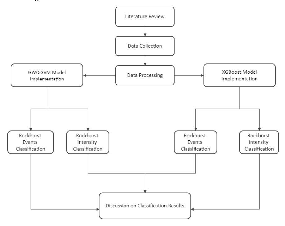
Research flow.
Grey Wolf Optimization – Support Vector Machine
In the GWO algorithm, the grey wolf population is divided into four classes based on the structure of its social hierarchy: alpha (), beta (), delta (), and omega (). The class is the leader, and its position is considered optimal for the algorithm. Meanwhile, and are determined as the second and third best solutions, respectively. The class is the candidate solution of all remaining wolves other than the previous three classes. During prey hunting, leads the search, whereas and assist in guiding . updates its position according to the position of , , and (see Figs. 2– 4 in Mirjalili et al. (2014) for the illustration).
In the GWO–SVM model, GWO plays a role in optimizing the parameters of the SVM: the parameter and the gamma parameter () on the radial basis function (RBF) kernel. Here, controls the trade-off between maximizing the margin and minimizing the classification error, whereas defines the influence range of a single training example in the RBF kernel. The optimization begins by initializing the positions of the grey wolves (candidate solutions) and evaluating their fitness, which is measured using the classification error of the SVM.
The process proceeds as follows:
1. Initialization: Set the initial positions of all wolves (possible parameter combinations for and ).
- 2. Fitness evaluation: Assess each wolf's performance based on SVM classification accuracy (lower error yields better fitness).
- 3. Position update: Adjust the positions of ω wolves according to the guidance of , , and using GWO's mathematical position-update rules.
- 4. Termination: Stop when the maximum number of iterations is reached or convergence is achieved.
The final output of GWO is the optimal pair of and , which is then applied to the SVM for rockburst classification. The detailed computational process of SVM can be found in Mirjalili et al. (2014), and the overall workflow of GWO– SVM is illustrated in Figure 3.
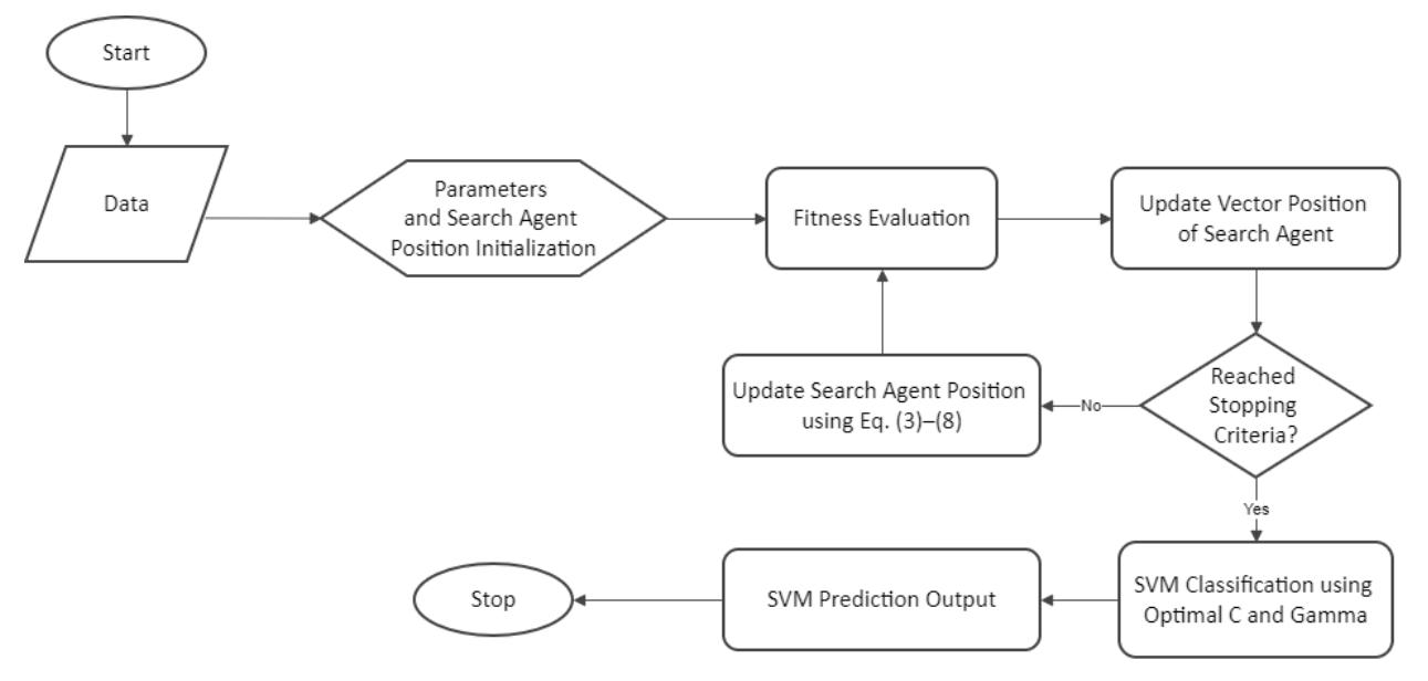
Flowchart of GWO-SVM.
To start the GWO process, we first initialize the parameters (grey wolf population, number of dimensions (in our case, 2, corresponding to and ), and number of iterations) and random positions for the search agent ( wolf) positions using Eq. (1):
\[\vec{X} = (upper\ bound - lower\ bound) \cdot \vec{r} + lower\ bound\] (1)
where ⃗ is the position vector of a search agent in the parameter space, the upper and lower bounds define the limit of the search space for each dimension, and is a vector with a random value in the interval (0, 1).
At each iteration , the fitness of each agent is evaluated using the classification error from SVM predictions (Eq. (2):
\[Fitness = 1 - accuracy (2)\]
A lower error indicates better suitability of the parameter combination. In updating the search agents' position, we use Eqs. (3) – (8). The distances between each wolf and the search agents are computed as follows:
\[\vec{D}_{\alpha} = \left| C_1 \cdot \vec{X}_{\alpha} - \vec{X} \right|, \ \vec{D}_{\beta} = \left| C_2 \cdot \vec{X}_{\beta} - \vec{X} \right|, \vec{D}_{\delta} = \left| C_3 \cdot \vec{X}_{\delta} - \vec{X} \right|\] \[(3)\] where ⃗ , ⃗ , and ⃗ represent the positions of the , , and wolves, respectively. ⃗ , ⃗ , and ⃗ are vectors representing the distances between the wolves and the search agents. 1 , 2 , and 3 are scalar coefficients controlling the step size of the search agents.
The new potential positions for the search agents are then updated as follows:
\[\vec{X}_1 = \vec{X}_{\alpha} - A_1 \cdot \vec{D}_{\alpha}, \quad \vec{X}_2 = \vec{X}_{\beta} - A_2 \cdot \vec{D}_{\beta}, \quad \vec{X}_3 = \vec{X}_{\delta} - A_3 \cdot \vec{D}_{\delta}\] \[\tag{4}\] where \(\vec{X}_1, \vec{X}_2\), and \(\vec{X}_3\) represent new potential positions for the search agents, respectively, which are influenced by the positions of \(\alpha\), \(\beta\), and \(\delta\). \(A_1\), \(A_2\), and \(A_3\) are scalar coefficients controlling the exploration or exploitation process. To calculate each \(A_i\) and \(C_i\), i=1,2,3 in Eqs. (3) – (4), we use Eqs. (5) – (7):
\[A_{i} = 2ar_{1} - a \tag{5}\]
\[C_{\rm i} = 2r_2 \tag{6}\]
\[a = 2 - 2\left(\frac{t}{max \ iteration}\right) \tag{7}\] where \(r_1\) and \(r_2\) are any random scalars in the interval (0, 1) and a is a random scalar coefficient with decreasing values from 2 to 0 during the iteration of \(r_1\) and \(r_2\). Finally, we can update the position of the search agents in the (t+1) iteration using Eq. (8):
\[\vec{X}(t+1) = \frac{\vec{X}_1 + \vec{X}_2 + \vec{X}_3}{3} \tag{8}\]
These steps are repeated until the stopping criterion (maximum iterations or convergence) is reached, producing the optimal pair \((C, \gamma)\) for SVM-based rockburst classification. At the end of the GWO process, we obtain the optimal values of parameter C and \(\gamma\) as the final position of \(\alpha\) \((\vec{X}_{\alpha})\), which serve as inputs of SVM.
We use a dataset with n=476 samples and m=6 features (see Table 1). Because y is a categorical variable (representing rockburst occurrence or intensity), it is encoded as a numerical value. For a given dataset, \(\mathcal{D}=\{(x_i,y_i)\}\) (\(|\mathcal{D}|=476\), \(x_i\in\mathbb{R}^6\), \(y_i\in\mathbb{R}\)), we use the RBF as our SVM kernel function, as given in Eq. (9):
\[K(\mathbf{x}_i, \mathbf{x}_j) = \exp\left(-\gamma \|\mathbf{x}_i - \mathbf{x}_j\|^2\right), \ \gamma > 0\] (9)
where \(x_i\) and \(x_j\) are six-dimensional feature vectors representing the observed mining conditions, and \(\gamma\) is the kernel width parameter optimized by GWO to control the influence range of each support vector. The penalty parameter C (also optimized by GWO) is applied in the dual formulation of the SVM optimization problem (see Hertono et al. (2024) for more details). The final equation of SVM is given by Eq. (10):
\[f(\mathbf{x}) = sgn(\sum_{i=1}^{n} [\lambda_i' y_i K(\mathbf{x}_i, \mathbf{x}_j)] + b'\] (10)
where \(\lambda_i'\) and b' are solutions that fulfill the Karush–Kuhn–Tucker conditions, \(K(x_i, x_j)\) is a kernel function, \(y_i\) is the target, and n is the number of support vectors. If the result of Eq. (10) is greater than 0, the data are classified as positive; otherwise, they are classified as negative.
Extreme Gradient Boosting
XGBoost is an ensemble learning algorithm developed from the GBDT algorithm. It is equipped with a regularization mechanism and column sampling method and adopts a parallel strategy in the DT splitting process, which greatly improves its speed and robustness (Zheng et al., 2023). Generally, it operates by creating an ensemble of DT, combining their predictions to make accurate classifications. Its process starts with the creation of a single DT, called a weak learner, which makes initial predictions. These predictions are then compared with the actual target values. The algorithm calculates the errors, highlighting where the model is making mistakes. In subsequent iterations, XGBoost builds additional trees, each focusing on reducing the errors made by previous ones. It assigns higher importance to misclassified data points, with the new trees designed to correct these errors. This iterative process continues until a predefined number of trees (or rounds) are built or until further tree additions do not significantly improve the model's performance.
In multiclass classification, XGBoost makes predictions using Eq. (11). For each class j, the predicted probability \(F_{ij}\) for the i-th input sample is calculated as follows:
\[F_{ii}(x_i) = F_0(x_i) + \sum_{k=1}^{K} f_{ik}(x_i)\] (11)
where \(F_0\) is the initial prediction score (set to zero for classification problems), K is the total number of DT, and \(f_{ik}(x)\) denotes the contribution of the k-th tree for the i-th observation and the input sample x. Thus, the final prediction is obtained by summing the outputs of all trees, which are sequentially added during the boosting process.
The algorithm of the XGBoost model is as follows:
1. Calculate the residual. The residual is the difference between the real value of the target variable and the initial predicted value, as given by Eq. (12):
\[residual_i = y_i - P_i \tag{12}\] where \(y_i\) represents the original value of the i-th data target variable and \(P_i\) represents the initial predicted probability of the positive class of i-th data for the first iteration. Generally, the initial predicted probability (\(P_0\)) of XGBoost is \(\frac{1}{m}\), with m being the number of classes.
- 2. Select an arbitrary feature for the start node and branch its nodes with other features.
- 3. Calculate the gain. The gain can be calculated from the difference between the objective function (we use log loss in this research) values before and after the split, as shown in Eq. (13):
\[gain = left_{similarity} + right_{similarity} - root_{similarity} - \gamma\] (13)
where \(\gamma\) is a regularization parameter with default value of 0, left or right similarity refers to the similarity score of the child node of a tree split, and root similarity refers to the similarity score of a root node. The similarity score in the Eq. (13) for the classification problems can be calculated using Eq. (14):
\[S_{j,k} = \frac{\left(\sum_{i=1}^{N} residual_{i,j,k}\right)^{2}}{\sum_{i=1}^{N} \left[P_{i,j,k} * (1-P_{i,j,k})\right] + \lambda}\] (14)
where \(residual_{i,j,k}\) is the residual of the i– th sample assigned to the split, \(P_{i,j,k}\) is its predicted probability, \(\lambda\) is the L2 regularization term to avoid overfitting with the default value zero, N is the total number of observations, and \(S_{j,k}\) is the similarity score of the leaf node-j and tree-k.
- 4. Pre-pruning (removing branches from a DT during tree-building to see if they provide little or no additional benefit). If the gain from a potential split is less than zero, the split is not performed. Instead, steps 2 and 3 are repeated, where the feature with the maximum gain is selected as the node split. These steps are repeated until no further branches can be formed for the tree.
- 5. Post-pruning (removing branches from a fully grown DT to see if they provide little or no additional benefit). If the gain is less than zero, the branch is pruned. Otherwise, the process proceeds to the next step.
- 6. Calculate the prediction output value for each leaf of tree-k using Eq. (15):
\[w_{j,k} = \frac{\sum_{i=1}^{N} residual_{i,j,k}}{\sum_{i=1}^{N} [P_{i,j,k}*(1-P_{i,j,k})] + \lambda}\](15)
Here, \(w_{i,k}\) represents the weight of leaf j in tree k, corresponding to the contribution of this leaf to the final prediction.
- 7. Perform steps 2 to 6 until the stopping criteria are met.
- 8. The prediction of tree-k can be calculated using Eq. (16):
\[f_k(\mathbf{x}) = \eta \cdot \sum_{j=1}^{J_k} \mathbf{w}_{j,k} \cdot \mathbf{I} \big( \mathbf{x} \in \mathbf{R}_{j,k} \big)\] (16)
where \(f_k(x)\) is the prediction of the k-th tree, \(\eta\) is the learning rate controlling the step size at each iteration, \(J_k\) is the total number of leaves in the tree-k, and \(I(x \in R_{j,k})\) is an indicator function that equals 1 if sample x falls into leaf j of tree-k, and 0 otherwise.
- 9. Update the prediction of XGBoost for each iteration using Eq. (11).
- 10. If the stopping criteria are not yet reached, update the residual for the next tree/iteration using Eq. (17):
\[residual_i^t = y_i - F_{t-1}(\mathbf{x}_i) \tag{17}\] where \(F_{t-1}\) represents the prediction of XGBoost at iteration t-1.
11. Repeat steps 2–10 until the stopping criteria are met. The final prediction of XGBoost is represented by the final result of Eq. (11).
Results
Computing Environment and Preprocessing
In this research, we used Python 3.9 as the programming language, executed through Google Colab. The device used was equipped with an Intel Core i3 Gen 11 processor (3 GHz, 4 CPUs) and 16 GB of RAM.
Before the implementation of these models, we implemented preprocessing steps on the dataset. There were some missing values in the initial dataset: 26 in MTS, UCS, and UTS and 2 in SC, RBC, ESI, and Intensity (see Table 1). We considered three imputation methods (mean, median, and mode) to handle the missing values. After the test, imputation using the mean gave the best result. Thus, we used mean imputation to handle the missing values in the initial dataset.
There were some outliers in the dataset, according to IQR checking. By testing two conditions (removing and retaining outliers), the model performed better after removing the outliers. As the feature range in our dataset varied, we decided to normalize them through min-max normalization. We compared the model's performance before and after normalization, with normalization yielding better results. Finally, to avoid model bias to a specific class, we performed SMOTE only on the training set. Obviously, this increased the number of data samples as we increased the number of minority classes. We also compared the model's performance before and after the SMOTE process. The results improved when we resampled the classes.
The rockbursts events and intensities were then classified using data that had passed all preprocessing stages (handling missing values and outliers, feature normalization, and data resampling). As GWO–SVM could produce optimal parameters, only the hyperparameters in XGBoost were tuned using GridSearchCV to obtain optimal parameters (see Table 3 for the range used).
Table 3 Hyperparameter range.
GWO-SVM XGBoost The search range of the number of iterations is 10–50 iterations, in increments of 10. The search range of the total population size of grey wolves is 10–50 wolves, in increments of 10. The number of dimensions is 2, as it relates to the optimization of the parameters C and gamma for SVM. The search range of the gamma value is the position of the grey wolf on the x-axis, which is searched within the range from 1–10 or 5–25. • The search range of the C value is the position of the grey wolf on the y-axis, which is searched within the range from 1–10 or 10–50. The search range of the learning rate (eta) is 0.01–1. This range is chosen so that the new trees added do not have too much or too little influence. The search range of gamma is 0.01–1. This range is chosen so that the minimum loss reduction from tree branching is neither too large nor too small. The search range of lambda is 0.01–1. This range is chosen so that the L2 regularization on each leaf weight is neither too large nor too small. The search range of the number of trees is 100–1000. The search range of the maximum depth of the trees is 6–10.
In this research, with the search ranges given in Table 3, we used the optimal value for each parameter in both models. For GWO–SVM parameters in event classification, we used 10 iterations, a grey wolf population size of 10, a gamma value of 8.5018, and a value of 34.113. In intensity classification, we used 10 iterations, a grey wolf population size of 40, a gamma value of 17.4008, and a value of 12.0328. For XGBoost parameters in event classification, we used 0.5 for the learning rate and gamma, 0.1 for lambda, 100 trees, and 10 for the maximum tree depth. In intensity classification, we used 0.1 for the learning rate and gamma, 0.5 for lambda, 1000 trees, and 8 for the maximum tree depth.
Figure 4 reveals the relationship between the six input features and the target variables (rockburst intensity and event occurrence). In this figure, darker colors represent stronger correlations (either positive or negative), whereas lighter shades indicate weaker relationships. Among all features, MTS, ESI, and SC exhibit the darkest shades with respect to the targets, confirming their dominant influence on rockburst classification. This observation aligns with the established rock mechanics theory, where stress concentration and brittleness are key triggers of rockburst events. In contrast, UCS and RBC appear lighter in the heatmap, indicating their relatively weaker contributions. Overall, the heatmap visually reinforces that MTS, ESI, and SC are the most critical predictors in modeling rockburst behavior
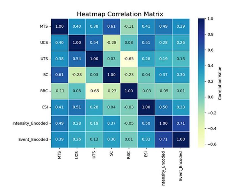
Heatmap correlation matrix.
GWO–SVM Performance for Rockburst Classification
The implementation of GWO–SVM was evaluated using various proportions of train–test split data: 50:50, 60:40, 70:30, 80:20, and 90:10. Each proportion was evaluated using various evaluation metrics and running time (average of five repetitions) for each proportion in the testing data. The rockburst events classification performance of GWO–SVM on the test set is shown in Table 4. Test set performance for rockburst event classification (GWO–SVM).
Table 4 Test set performance for rockburst event classification (GWO–SVM).
| Evaluation Metrics | |||||
|---|---|---|---|---|---|
| Train–Test Split | Accuracy (%) | Precision (%) | Recall (%) | F1-Score (%) | Running Time (s) |
| 50:50 | 92.611 | 87.339 | 86.488 | 86.905 | 3.468 |
| 60:40 | 93.210 | 86.008 | 89.445 | 87.593 | 3.598 |
| 70:30 | 95.082 | 91.372 | 91.372 | 91.372 | 3.602 |
| 80:20 | 97.531 | 94.444 | 98.462 | 96.278 | 4.218 |
| 90:10 | 100 | 100 | 100 | 100 | 4.952 |
Note. Metrics reported: accuracy, precision, recall, F1-score, and runtime (s). Numbers in bold are the best values per column. The results are averaged over five runs. SMOTE was applied to the training split only.
Subsequent analyses used the 80:20 train–test split. The 90:10 split yielded a lower test performance alongside higher training scores, indicating overfitting. At 80:20, the event classification shows had comparable training and test metrics, suggesting no overfitting under this setting. Performance improved as the training fraction increased from 50:50 to 80:20. The GWO–SVM test set results for intensity classification are reported in Table 5.
Table 5 Test set performance for rockburst intensity classification (GWO-SVM).
| Evaluation Metrics | |||||||
|---|---|---|---|---|---|---|---|
| Train–Test Split | Accuracy (%) | Precision (%) | Recall (%) | F1-Score (%) | Running Time (s) | ||
| 50:50 | 70.000 | 67.787 | 68.965 | 68.325 | 3.252 | ||
| 60:40 | 70.588 | 67.301 | 74.131 | 69.064 | 3.750 | ||
| 70:30 | 72.549 | 67.828 | 72.652 | 68.681 | 4.682 | ||
| 80:20 | 80.882 | 78.862 | 80.141 | 79.322 | 5.638 | ||
| 90:10 | 85.294 | 85.880 | 89.286 | 84.138 | 5.484 | ||
Note. Metrics reported: accuracy, precision, recall, F1-score, and runtime (s). Numbers in bold are the best values per column. The results are averaged over five runs. SMOTE was applied to the training split only.
Subsequent intensity analyses used the 90:10 train–test split. At 90:10, the training and test metrics were comparable, indicating no overfitting under this setting. Across splits, performance increased as the training fraction rose from 50:50 to 90:10. Comparing the best results in Table 4 (event) and Table 5 (intensity), the intensity metrics were lower than the event metrics.
XGBoost Performance for Rockburst Classification
The same procedures as in GWO–SVM were applied in the implementation of XGBoost. The rockburst event classification performance of XGBoost on the test set is shown in Table 6. In Table 6, the best event classification performance for XGBoost occured at the 80:20 train–test split. This was consistent with GWO–SVM, whose best event result also appeared at 80:20. Accordingly, we used the 80:20 split for subsequent event analyses. Performance increased monotonically from 50:50 to 80:20 and decreased at 90:10. At 80:20, XGBoost's inference time was 0.545s versus 4.218s for GWO–SVM (approximately eight times faster).
Train–Test Split Evaluation Metrics Accuracy (%) Precision (%) Recall (%) F1-Score (%) Running Time (s) 50:50 60:40 70:30 80:20 90:10 91.133 91.358 91.803 97.531 92.683 83.321 82.344 84.454 94.444 91.319 88.988 88.350 89.392 98.462 88.387 85.718 84.888 86.605 96.278 89.724 0.856 0.656 0.523 0.545 0.747
Table 6 Test set performance for rockburst event classification (XGBoost)
Note. Metrics reported: accuracy, precision, recall, F1-score, and runtime (s). Numbers in bold are the best values per column. The results are averaged over five runs. SMOTE was applied to the training split only.
The intensity classification results for XGBoost on the test set are reported in Table 7.
| Evaluation Metrics | |||||||
|---|---|---|---|---|---|---|---|
| Train–Test Split | Accuracy (%) | Precision (%) | Recall (%) | F1-Score (%) | Running Time (s) | ||
| 50:50 | 62.353 | 59.336 | 62.754 | 60.287 | 1.703 | ||
| 60:40 | 64.706 | 61.274 | 67.081 | 62.533 | 0.106 | ||
| 70:30 | 68.628 | 63.736 | 67.588 | 64.430 | 0.656 | ||
| 80:20 | 76.471 | 73.362 | 79.438 | 73.535 | 0.291 | ||
| 90:10 | 88.235 | 84.127 | 91.369 | 86.508 | 1.910 | ||
Table 7 Test set performance for rockburst intensity classification (XGBoost).
Note. Metrics reported: accuracy, precision, recall, F1-score, and runtime (s). Numbers in bold are the best values per column. The results are averaged over five runs. SMOTE was applied to the training split only.
According to evaluation metrics, the 90:10 train–test split yielded the best performance for rockburst intensity using XGBoost, consistent with GWO–SVM. Accordingly, subsequent intensity analyses used the 90:10 split. Across splits, performance improved as the training fraction increased from 50:50 to 90:10. In terms of runtime, XGBoost executed longer on the intensity task than on the event (binary) task.
Discussion
A comparative analysis between GWO–SVM and XGBoost was conducted by evaluating the best-performing results across both models. The comparison first considered the confusion matrices of rockburst event classification with an 80:20 train–test split and rockburst intensity classification with a 90:10 train–test split. For rockburst event classification, the test set consisted of 81 observations (20%), whereas the test set for the rockburst intensity classification comprised 34 observations (10%). The detailed results of these confusion matrices are presented in Tables 8 and 9, respectively.
The confusion matrices presented in Table 8 demonstrate that both GWO–SVM and XGBoost achieved identical outcomes for rockburst event classification. All 16 "Existent" events were correctly classified, whereas only two instances of "None" were misclassified as "Existent". This indicated the absence of false negatives a critical requirement in rockburst prediction tasks, as missing an actual event may lead to catastrophic consequences. Although the occurrence of a few false positives could result in unnecessary alarms, such outcomes are generally more tolerable in the mining safety domain compared with the risks posed by false negatives.
| Table 8 | Confusion matrices for rockburst event classification using GWO–SVM and XGBoost on test sets. |
|---|
| GWO–SVM | XGBoost | ||||||
|---|---|---|---|---|---|---|---|
| Predicted | Predicted | ||||||
| Actual | Existent | None | Actual | Existent | None | ||
| Existent | 16 | 0 | Existent | 16 | 0 | ||
| None | 2 | 63 | None | 2 | 63 | ||
Table 9 highlights the classification results for rockburst intensity, where both models demonstrated strong predictive capacity. However, in contrast to event classification, intensity prediction was more challenging. XGBoost showed a slightly better consistency across multiple intensity levels compared with GWO–SVM, reducing misclassifications among adjacent classes. This aligns with prior studies (Xue et al., 2020; Wang et al., 2022; Wojtecki et al., 2021) that emphasized that ensemble-based models often perform more robustly in multiclass problems given their ability to capture complex feature interactions. Nonetheless, some overlap among classes persisted, indicating that further feature engineering or hybrid modeling may be required for improved performance in rockburst intensity prediction.
Table 9 Confusion matrices for rockburst-intensity classification using GWO–SVM and XGBoost on test sets.
| GWO–SVM XGBoost | ||||||||
|---|---|---|---|---|---|---|---|---|
| Predicted | Predicted | |||||||
| Actual | Weak | Moderate | Strong | Actual | Weak | Moderate | Strong | |
| Weak | 13 | 1 | 0 | Weak | 13 | 1 | 0 | |
| Moderate | 2 | 12 | 2 | Moderate | 1 | 13 | 2 | |
| Strong | 0 | 0 | 4 | Strong | 0 | 0 | 4 | |
Table 10 compares the evaluation metrics in rockburst event classification between GWO–SVM and XGBoost models using 80% of the training data.
Table 10 Comparison of the rockburst event classification performances of GWO–SVM and XGBoost on test sets with 80% training data.
| Evaluation Metrics | |||||
|---|---|---|---|---|---|
| Model | Accuracy (%) | Precision (%) | Recall (%) | F1-Score (%) | Running Time (s) |
| GWO–SVM | 97.531 | 94.444 | 98.462 | 96.278 | 4.218 |
| XGBoost | 97.531 | 94.444 | 98.462 | 96.278 | 0.545 |
The results in Table 10 confirm that both models achieved equivalent predictive performance, with high accuracy (97.53%), precision (94.44%), recall (98.46%), and F1-score (96.28%). However, the key distinction lies in computational efficiency. GWO–SVM required 4.218s to complete the task, whereas XGBoost completed it in only 0.545s. This discrepancy could be attributed to the algorithmic complexity of each method. GWO–SVM integrates the grey wolf optimizer, which iteratively searches for optimal SVM hyperparameters through repeated kernel evaluations, leading to higher computational cost. In contrast, XGBoost leverages an efficient histogram-based GB framework and parallelized tree construction, both of which scale more linearly with dataset size. These algorithmic differences explain why XGBoost is substantially faster, highlighting its practical advantage for real-time monitoring applications where rapid response is critical.
Table 11 summarizes the comparison of evaluation metrics in rockburst intensity classification by both GWO–SVM and XGBoost models using 90% of the training data.
Table 11 Comparison of the rockburst intensity classification performances of GWO–SVM and XGBoost on test sets with 90% training data.
| Evaluation Metrics | ||||||
|---|---|---|---|---|---|---|
| Model | Accuracy (%) | Precision (%) | Recall (%) | F1-Score (%) | Running Time (s) | |
| GWO-SVM | 85.294 | 85.880 | 89.286 | 84.138 | 5.484 | |
| XGBoost | 88.235 | 84.127 | 91.369 | 86.508 | 1.910 | |
The comparative results in Table 11 emphasize the greater challenge of rockburst intensity classification. Although GWO–SVM and XGBoost both achieved high predictive metrics, XGBoost outperformed GWO–SVM in terms of recall (91.37% vs. 89.29%) and F1-score (86.51% vs. 84.14%). The running time further illustrated the computational gap: GWO–SVM took 5.484s, whereas XGBoost completed the task in only 1.910s. The slower performance of GWO–SVM
stemmed from its reliance on metaheuristic optimization and computationally expensive SVM kernel evaluations, both of which scale poorly as the complexity of the classification task increased. In contrast, XGBoost benefited from optimized GB with parallel computation and efficient memory usage, enabling it to handle imbalanced multiclass data more effectively with reduced latency. These results suggest although both models are accurate, XGBoost offers superior feasibility for operational decision-making in mining environments, where rapid detection and response are essential for safety. Table 12 shows the performances of both models in predicting each class of rockburst events class rockburst events.
Table 12 Class prediction in rockburst event classification by both models.
| GWO–SVM | XGBoost | |||||
|---|---|---|---|---|---|---|
| Class | Precision | Recall | F1-Score | Precision | Recall | F1-Score |
| None | 0.89 | 1.00 | 0.94 | 0.89 | 1.00 | 0.94 |
| Exist | 1.00 | 0.97 | 0.98 | 1.00 | 0.97 | 0.98 |
The results in Table 12 highlight the class-level performance of both models for rockburst events. The Existent class achieved perfect precision (1.00) in both models, indicating that all events predicted as Existent were indeed true positives. However, the recall for this class was slightly lower (0.97), reflecting a small number of false negatives. In contrast, the None class demonstrated perfect recall (1.00) but lower precision (0.89), showing that some negative cases were misclassified as events. This trade-off indicates that both models prioritize minimizing false negatives for the None class, which is crucial for safety in rockburst monitoring applications. Missing a true rockburst event can have severe consequences, whereas occasionally false alarms are generally more acceptable in operational settings. Overall, the F1 score values (0.98 for Existent and 0.94 for None) confirm that the models maintain a balanced and reliable classification across both classes, with slightly stronger emphasis on detecting actual rockburst occurrences. Table 13 shows the performances of both models in predicting each class in rockburst intensity classification.
Table 13 Class prediction in rockburst intensity classification by both models.
| GWO–SVM | XGBoost | ||||||
|---|---|---|---|---|---|---|---|
| Class | Precision | Recall | F1-Score | Precision | Recall | F1-Score | |
| Weak | 0.87 | 0.93 | 0.90 | 0.93 | 0.93 | 0.93 | |
| Moderate | 0.92 | 0.75 | 0.83 | 0.93 | 0.81 | 0.87 | |
| Strong | 0.67 | 1.00 | 0.80 | 0.67 | 1.00 | 0.80 | |
Overall, both models had a better evaluation of the "Weak" class than the "Moderate" and "Strong" classes. Although the "Strong" class had erfect recall for both models, its precision was low. In the context of rockbursts, precision refers to the proportion of correctly identified rockburst events (true positives) out of all instances predicted as rockbursts. We suspect that this low precision value was due to an imbalance in the testing data, thus limiting the model's ability to learn from the data in determining the proportion of correctly identified rockburst events (true positive) out of all instances predicted as strong rockbursts. This was evidenced by the low precision value (0.67) on the Strong class in both models.
Recall measured the models' ability to detect all actual rockburst events, indicating the proportion of true rockbursts that were correctly classified. Data imbalance in testing data might have limited the models' ability to detect all actual rockbursts in the Moderate class. This was shown by the low recall value in the Moderate class (0.75 and 0.81 for GWO– SVM and XGBoost, respectively). The F1-score balanced precision and recall, providing an overall measure of the models' effectiveness in correctly identifying rockbursts without overlooking too many or making too many false predictions. From the results, XGBoost achieved a precision, recall, and F1-score of 0.93 in predicting the Weak class. A precision of 0.93 means that 93% of the cases that the model classified as rockbursts were in fact rockbursts. The model rarely made false positive predictions, indicating its ability to avoid misclassifying nonrockburst events as rockbursts. A recall of 0.93 means that the model correctly identified 93% of the actual rockbursts. The model effectively captured almost all true rockburst events, with a low rate of false negatives (i.e., missing true rockbursts). Lastly, a score of 0.93 for the F1-score means that the model maintained a good balance between precision and recall. The model was good at both identifying rockburst events and avoiding incorrect classifications, resulting in a strong overall classification performance. Because both models are better at predicting the "Weak" class, it becomes our limitation when building a model that can predict the "Strong" class better than the rest of the classes.
When compared with previous research (Li et al., 2023) that used GWO–SVM, with more observations, this research proves that classifying rockburst events and intensity can work very well with GWO–SVM. The results show a positive effect in handling imbalanced data on classification performance. By balancing the target classes in the training set, the model is more predictive and therefore performs classification better. With a much larger number of observations, this research also validates the results of He et al. (2023) who had excellent performance results on rockburst intensity classification problems using XGBoost. By integrating oversampling strategies with larger datasets, the present study provides stronger evidence that both GWO-SVM and XGBoost are viable for rockburst prediction, while highlighting the need for further methodological improvements, such as hybrid resampling, cost-sensitive learning, or feature engineering to enhance discrimination, particularly for the Strong class. Table 14 compares the results of this research with those of research that used other optimizers.
| Model | Test sets correct rate (%) | Reference | |
|---|---|---|---|
| 85.29 | |||
| GWO–SVM | (29/34) | This paper | |
| 88.24 | |||
| XGBoost | (30/34) | This paper | |
| 77.78 | |||
| PSO–SVM | (7/9) | (Zhou et al., 2012) | |
| 77.78 | |||
| GA–SVM | (7/9) | (Zhou et al., 2012) | |
Table 14 Comparison of rockburst intensity classification performances.
As shown in Table 14, GWO–SVM and XGBoost achieved superior test set performance compared with previous optimization-based SVM approaches, such as particle swarm optimization–SVM (PSO–-SVM) and genetic algortihm– SVM (GA–SVM), which reported 77.78% accuracy with a smaller test set of nine instances. With the higher number of observations (34) in the test set, this study achieved higher accuracies of 85.29% and 88.24% for GWO–SVM and XGBoost, respectively. The values (29/34) and (30/34) show the number of correct predictions over the total number of observations in the test set.
Given its high accuracy and low latency, XGBoost is well-suited for early warning and mitigation of rockbursts, helping reduce operational risks and potential losses. To strengthen field deployment, future work should refine Strong-class precision via cost-aware thresholding and hybrid resampling, incorporate physics-informed features, and perform validation across multiple sites with uncertainty and explainability reporting.
Conclusion
This study addressed the prediction of rockburst occurrences (events) and rockburst intensities in underground mines using GWO–SVM and XGBoost. With standardized preprocessing and split evaluations, both models performed strongly for event classification at the 80:20 split, each achieving 97.53% accuracy, 0.9444 precision, 0.9846 recall, and 0.9628 F1-score. For intensity classification at 90:10, XGBoost outperformed GWO–SVM in terms of accuracy, recall, F1-score, and runtime (accuracy, 88.24%; precision, 0.8413; recall, 0.9137; F1-score, 0.8651). Class-wise analysis indicated that predictions were most reliable for the Weak class. Meanwhile, the Moderate class showed lower recall and the Strong class suffered from lower precision—patterns consistent with residual class imbalance and feature overlap. Overall, these results confirm the promise of combining optimization-based SVM and ensemble learning for rockburst prediction, with XGBoost particularly suitable for early warning scenarios given its lower latency. Future work should prioritize hybrid resampling and cost-sensitive/threshold tuning to improve Strong-class precision, explore physicsinformed and spatiotemporal features, and conduct multisite external validation with uncertainty and explainability reporting to strengthen robustness and field deployment.
Acknowledgment
This research was fully supported by the FMIPA Universitas Indonesia Research Grant No. NKB-018/UN2.F3.D/PPM.00.02/2023.
Compliance with ethics guidelines
The authors declare they have no conflict of interest or financial conflicts to disclose.
This article contains no studies with human or animal subjects performed by the authors.