
Introduction
In recent decades, four-rotor unmanned aerial vehicles (UAVs), commonly referred to as quadcopters, have garnered significant attention in the literature due to their low cost, vertical take-off and landing (VTOL) capabilities, and simple design and manufacturing process compared to their fixed-wing counterparts. The aforementioned features have made them an indispensable aerial vehicle in a wide range of applications in numerous fields. Consequently, they can be implemented in a broad spectrum of applications, including agriculture, industry, military surveillance and reconnaissance, commerce, search and rescue missions, and even everyday life activities. Furthermore, they perform various tasks, including crop monitoring, fertilization, spraying, aerial terrain mapping, power line maintenance, cargo transportation, and more (Cardenas and De Barros, 2019). In fact, the foundation for effectively accomplishing the previously mentioned specialized tasks is the accurate trajectory tracking control system. However, the inherent nonlinearity associated with the UAV's dynamic nature, alongside the uncertainties arising from the complexity of capturing a precise model for an aerodynamic-structural interacting system, is a challenge. As a result, the development of navigation systems, position estimation, flight stability, and several other control tasks is significantly affected. Subsequently, extensive research efforts have been dedicated to addressing these challenges through proposing numerous control system strategies. These include Proportional-Integral-Derivative (PID) controllers, adaptive nonlinear control, feedback linearization control, and other model-based control systems.
The backstepping is a recursive control technique with a key advantage of handling complex and nonlinear systems. It tackles such systems by decomposing them into subsystems, which are subsequently managed iteratively via Lyapunov functions as well as intermediate virtual controls. This framework ensures improved control performance and system stability. However, the backstepping method, in its basic form, lacks the robustness property against uncertainties and external disturbances. On the other hand, sliding mode variable structure control exhibits adaptability, robustness, and rapid convergence even in the presence of parameter uncertainties and external interference. Consequently, researchers often integrate sliding mode control with backstepping to enhance the system's anti-interference capabilities (Zhang et al., 2023; Zinober, 2005).
The hybridization of sliding mode and backstepping control has produced robust control strategies with smooth control inputs for nonlinear systems (Li and Zhang, 2017). For instance, a stability control strategy for four-rotor UAVs based on an integral backstepping control was found to achieve improved stability and accuracy under external torque disturbances (Huo, Huo and Karimi, 2014). In addition, a feedback linearization controller was proposed for a quadrotor UAV with tiltable rotors to ensure trajectory tracking under gust disturbances (Saif, 2017). As illustrated in (Pang, Zhang and Xu, 2018) and (Huang, Zhang and Sun, 2019), improved backstepping methods have addressed challenges such as parameter tuning and large tracking errors in nonlinear mechanical systems. To enhance tracking accuracy, Ali et al. (2019) proposed adaptive backstepping sliding mode schemes for a coaxial multi-rotor UAV. Moreover, techniques such as differential evolution optimization (Mousa and Hussein, 2022) and neural network integration (Jiang, Pourpanah, and Hao, 2019) have further enhanced the robustness and anti-interference capabilities of UAV control systems. Also, a robust adaptive integral terminal sliding mode control was introduced in (Labbadi and Cherkaoui, 2019) to address position tracking convergence issues in the presence of model uncertainties and external disturbances.
While sliding mode control excels in handling parameter uncertainties and external disturbances, the discontinuity of the sliding surface, combined with the controller's fast response, often leads to chattering. Common solutions to mitigate chattering include replacing the discontinuous sign function with smoother alternative functions, such as saturation or hyperbolic tangent functions. Nonetheless, these adjustments may compromise the robustness of the system and increase the closed-loop system's sensitivity to unmodeled dynamics. An alternative solution involves integrating fractional-order calculus with sliding mode control (Jinkun, 2011). Fractional calculus extends traditional calculus by incorporating time-memory effects while enhancing robustness. This theory, which originated in 1695, has undergone substantial evolution and gained widespread applications through the dedicated efforts of numerous researchers. In fact, incorporating fractional calculus into the controller design framework enhances flexibility because fractional-order operators more accurately describe the dynamic behaviors of systems. Compared to integer-order approaches, fractional-order controllers offer superior closed-loop characteristics, thereby enhancing the stability and reliability of controlled systems (Yang and Xue, 2017). Podlubny's groundbreaking work (Podlubny, 1999) transitioned traditional PID control to fractional-order PID (FOPID), leading to significant advancements in automatic control theory. Subsequent studies have explored fractional-order sliding mode control to address nonlinear system disturbances and improve robustness (Al-Dhaifallah et al., 2023). For instance, fuzzy controllers (Mofid, Mobayen and Wong, 2020) and innovative fractional sliding surfaces (Rao et al., 2022) have been proposed to reduce chattering while enhancing performance. Applications of fractional-order control also extend to specialized systems, such as quadrotors with slung loads (Ferik et al., 2023) and ship navigation (Li et al., 2020), where these methods improve tracking accuracy, robustness, and response times.
Recently, several SMC-based controllers have been proposed to improve the quadcopter trajectory tracking performance (Elagib and Karaarslan, 2023). Jing integrated an SMC with a disturbance observer for a quadrotor subjected to disturbances and in a turbulent indoor space (Jing et al., 2023). Nguyen introduced an integral terminal sliding mode fault-tolerant controller, which actively addresses disturbances, saturation, and fault issues (Nguyen and Pitakwachara, 2024). To improve the trajectory tracking of quadcopters, Gedefaw and his team proposed a novel SMC with a fuzzy PID surface under external disturbances (Gedefaw et al., 2024, 2025). For a fixed-wing UAV, Metekia utilized fractional calculus theory to develop a robust fractional order SMC, with its gains optimized using Particle Swarm Optimization (PSO) (Metekia et al., 2025). Moreover, for a fixed-wing UAV, Mohammed utilized adaptive control theory to stabilize the vehicle under external disturbances (Mohammed et al., 2025), while Yashede employed a Neuro-Fuzzy Inference System-based Sliding Mode Controller to address the same problem (Yashede et al., 2025). Finally, Abera et al. (2024) presented a robust enhanced nonsingular adaptive super twisting SMC for tracking of a quadrotor under external disturbances and model uncertainties.
This work leverages the strengths of both Lyapunov-based nonlinear control and adaptive sliding mode control. The proposed controller is capable of tracking desired flight paths with a high level of accuracy while ensuring minimal adjustment time. Specifically, the contributions of the current research are to introduce a novel hybrid nonlinear control method for four-rotor UAVs in the presence of external disturbances. This hybrid control approach effectively addresses the challenges associated with the nonlinear dynamics and uncertainties inherent in four-rotor UAV systems, providing
improved stability and performance. In addition, unlike the simplified linear models, the proposed controller expands the validity of the control-oriented model by incorporating the nonlinearities associated with the interactions among the degrees of freedom. The structure of this paper is organized as follows: The dynamic model of the four-rotor UAV is presented in detail in the second section, providing a thorough understanding of the system's behavior and motion. To ensure stable flight control and reliable trajectory tracking performance, the third section presents the controller design for the position and attitude subsystems. Additionally, the stability of the suggested nonlinear control approach is thoroughly demonstrated using the Lyapunov stability theory. The efficacy and versatility of the proposed controller are demonstrated under various conditions in the fourth section, which presents the results of simulations for different flight trajectories of the four-rotor UAV. The paper concludes in the fifth section, where possible avenues for future research are highlighted, summarizing the main conclusions and implications of this study.
Dynamic Model of Quadcopter UAV
The physical structure of a typical quadcopter, a prevalent configuration of an unmanned aerial vehicle (UAV), is illustrated in Figures 1 and 2. To define its motion, two primary coordinate systems are predominantly employed: the body-fixed coordinate system (B), which is attached to the quadcopter's frame and moves with it, and the Earth-fixed inertial coordinate system (I) (Sabatino, 2015; Niu et al., 2022).To derive the governing equations of motion for the UAV, the following underlying assumptions are introduced.
- 1. The four-rotor UAV is treated as a rigid body in this study.
- 2. The center of mass of the UAV is coincident with the vehicle body-fixed frame.
- 3. The lift force induced by the propeller is proportional to the square of the propeller's rotational speed.
A flying quadcopter has six degrees of freedom (DoF), which encompass both translational and rotational movements. The quadcopter's linear location is determined by translational motion along the X, Y, and Z axes, which are denoted by the letters x, y, and z, respectively. φ (roll), θ (pitch), and ψ (yaw) are the angular locations that arise from the rotational motion about these axes. In particular:
- : Rotation about the -axis (roll).
- : Rotation about the -axis (pitch).
- : Rotation about the -axis (yaw).
Figure 1 A quadcopter. Figure 2 Quadcopter physical structure.
Together, these translational and rotational components define the quadcopter's orientation and position in threedimensional space. The dynamics of the quadcopter are governed by a set of coupled nonlinear equations that reflect its translational and rotational behaviors. This dynamical representation considers the interplay of forces and moments acting on the UAV, ensuring an accurate description of its flight characteristics. The mathematical formulation of these dynamics is expressed in Eq. 1 (Sabatino, 2015; Niu et al., 2022; Muliadi and Kusumoputro, 2018; Sari and Darwito, 2024). The aforementioned equations form the basis for the development of controllers capable of precise trajectory tracking, enhancing flight stability, and improving robustness against external disturbances.
A thorough understanding of the quadcopter's physical structure, coordinate systems, and dynamic equations is crucial for developing advanced control strategies. By leveraging these principles, innovative control methods can be implemented to optimize the quadcopter's performance in diverse applications, including aerial monitoring, cargo delivery, and search-and-rescue operations.
\[\ddot{x} = \frac{U_1}{m} [\cos \phi \cos \psi \sin \theta + \sin \phi \sin \psi] - \frac{k_1}{m} \dot{x} + d_1\]
\[\ddot{y} = \frac{U_1}{m} [\cos \phi \cos \psi \sin \theta + \sin \phi \sin \psi] - \frac{k_2}{m} \dot{y} + d_2\] \[\ddot{z} = \frac{U_1}{m} [\cos \phi \cos \theta] - g - \frac{k_3}{m} \dot{z} + d_3\] \[\ddot{\phi} = \dot{\theta} \dot{\psi} \left( \frac{l_y - l_z}{l_x} \right) + \frac{l_r \omega_r}{l_x} + \frac{lU_2}{l_x} - \frac{lk_4}{l_x} \dot{\phi}\] \[\ddot{\theta} = \dot{\theta} \dot{\psi} \left( \frac{l_z - l_x}{l_y} \right) - \dot{\phi} \frac{J_r \omega_r}{l_x} + \frac{lU_3}{l_y} - \frac{lk_5}{l_x} \dot{\theta}\] \[\ddot{\psi} = \dot{\theta} \dot{\phi} \left( \frac{l_x - l_y}{l_z} \right) + \frac{CU_4}{l_z} - \frac{lk_6}{l_x} \dot{\psi}\] \[(1)\]
The parameters defining the quadcopter dynamics include several critical components essential for modeling and control. The rotor's moment of inertia is denoted by \(J_r\), while the quadcopter's arm length is represented by l. The symbols \(I_x\), \(I_y\), and \(I_z\). The aerodynamic friction coefficient is expressed as \(k_i\) and C refers to the proportional coefficient of the force moment. Additionally, \(d_i\) represents external disturbances acting on the system. The control inputs of the system, which are directly influenced by the angular velocities of the quadcopter's four rotors, are given as \(U_1\), \(U_2\), \(U_3\), and \(U_4\). These inputs are mathematically formulated and expressed in Eq. (2), encapsulating the relationship between rotor dynamics and control actions.
\[\begin{bmatrix} U_1 \\ U_2 \\ U_3 \\ U_4 \end{bmatrix} = \begin{bmatrix} k_t & k_t & k_t & k_t \\ k_t & 0 & -k_t & 0 \\ 0 & -k_t & 0 & k_t \\ -k_b & k_b & -k_b & k_b \end{bmatrix} \begin{bmatrix} \omega_1^2 \\ \omega_2^2 \\ \omega_3^2 \\ \omega_4^2 \end{bmatrix}\](2)
\(k_t\) and \(k_b\) are the thrust and drag coefficients, respectively. \(\omega_r\) is the linear combination of the speeds of the four rotors (see Eq. (3)).
\[\omega_r = -\omega_1 + \omega_2 - \omega_3 + \omega_4 \tag{3}\]
Controller Design
Four-rotor UAVs predominantly use positioning tracking for flight control, and maintaining their in-flight stability is heavily dependent on attitude control. Thus, this study proposes a novel nonlinear hybrid approach that enhances, to some extent, the system's tracking accuracy, resilience, and control flexibility.
In this paper, both Lyapunov and adaptive sliding mode control methods equally strive to achieve the desired tracking, as shown in the block diagram (Figure 3). The proposed method utilizes adaptive sliding-mode control (ASMC) specifically for the quadcopter's position dynamics. Unlike standard SMC, our approach utilizes an adaptive law to estimate and compensate for unknown external disturbances that impact the system's performance. The control inputs \(v_1\) and \(v_2\), as will be shown, are generated by this adaptive law for the x and y axes, respectively. This adaptive mechanism distinguishes our approach from conventional SMC by eliminating the need for a priori knowledge of disturbance bounds, thereby enhancing robustness and tracking accuracy.
Additionally, the inherent robustness built into the paradigm of the sliding mode controller holds for any bounded disturbance (constant or time varying). However, incorporating wind disturbances will reinforce the evaluation of the proposed controller's robustness.
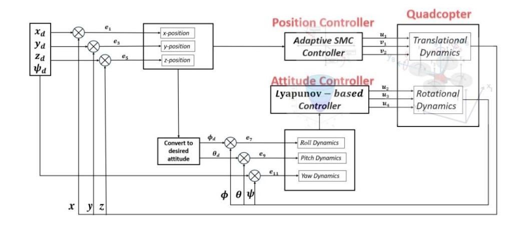
Figure 3 Control system block diagram.
Position Control
The four-rotor UAV's position controller utilizes control input, 1 , to determine the thrust demand from each rotor. The variation of the thrust induced among the rotors enables the controller to regulate the UAV's acceleration in all directions.
For the position control, the following equations are extracted from Eq. (1)
\[\ddot{x} = \frac{U_1}{m} [\cos \phi \cos \psi \sin \theta + \sin \phi \sin \psi] - \frac{k_1}{m} \dot{x} + d_1\] \[\ddot{y} = \frac{U_1}{m} [\cos \phi \cos \psi \sin \theta + \sin \phi \sin \psi] - \frac{k_2}{m} \dot{y} + d_2\] \[\ddot{z} = \frac{U_1}{m} [\cos \phi \cos \theta] - g - \frac{k_3}{m} \dot{z} + d_3\]
The dynamic model in the altitude direction can be written as in Eq. (4):
\[z_1 = z\]
\(\dot{z}_1 = z_2\)
\(\ddot{z}_2 = \frac{U_1}{m} [\cos \phi \cos \theta] - g - \frac{k_3}{m} z_2 + d_3\) (4)
Moreover, error dynamics are defined in Eq. (5).
\[e_{5} = z_{1} - z_{1d}\] \(e_{6} = \dot{z}_{1} - \dot{z}_{1d}\) \(\dot{e}_{5} = e_{6}\) \(\dot{e}_{6} = \dot{z}_{2} - \ddot{z}_{2d}\) (5)
In the framework of the sliding mode controller, the following sliding surface is considered:
\[\sigma_{3} = \lambda_{3}e_{5} + e_{6}\] \[\dot{\sigma}_{3} = \lambda_{3}\dot{e}_{5} + \dot{e}_{6}\] \[\dot{\sigma}_{3} = \lambda_{3}e_{6} + \dot{e}_{6}\] \[\dot{\sigma}_{3} = \lambda_{3}e_{6} + \dot{z}_{2} - \ddot{z}_{2d}\] \[(6)\]
Theorem 1: The control law defined by the equation
\[U_1 = \frac{m}{\cos\phi\cos\theta} \left(g + \frac{k_3}{m}z_2 - \lambda_3 e_6 + \ddot{z}_{1d} - M_3 \operatorname{sign}(\sigma_3)\right)\] is able to stabilize the nonlinear dynamical subsystem governed by Eqs. (4)-(6) in a finite time if and only if 3 > 0 and 3 > 3 .
Proof 1: The following positive definite Lyapunov function candidate is introduced:
\[\begin{split} V_3 &= \frac{1}{2}\sigma_3^2 \\ \dot{V}_3 &= \sigma_3 \, \dot{\sigma}_3 \\ \dot{V}_3 &= \sigma_3 |\lambda_3 e_6 + \frac{u_1}{m} \cos\phi \, \cos\theta - g - \frac{k_3}{m} z_2 + d_3 - \ddot{z}_{1d}| \, (7) \end{split}\]
To guarantee stability in the Lyapunov sense, it is required to have a negative definite or at least a negative semi-definite time derivative of the Lyapunov energy function. One may be able to devise the control law such that \(V_3 < 0\). Choose \(U_1 = \frac{m}{\cos\phi\,\cos\theta}\,\,(g + \frac{k3}{m}\,z_2 \,-\,\lambda_3 e_6 \,+\, \ddot{z}_{1d} - M_3\,sign(\sigma 3)).\) \(D_3\) is the maximum value of external disturbance and \(M_3\) is a positive constant \(M_3 > D_3\). It is important to distinguish between the disturbance value \(d_i\) and the maximum possible disturbance value \(D_i\). The Lyapunov function is written as:
\[\dot{V}_3 = \sigma_3(-M_3 \operatorname{sign}(\sigma_3) + d_3) = -M_3|\sigma_3| + \sigma_3 d_3 \le -M_3|\sigma_3| + |\sigma_3|D_3 = -|\sigma_3|(M_3 - D_3) \quad \blacksquare\] (8)
Since the term \((M_3 - D_3)\) is positive, then \(\dot{V}_3 \le -(M_3 - D_3)|\sigma_3|\) or \(\dot{V}_3 \le -(M_3 - D_3)\sqrt{2}V^{1/2}\). For a trajectory starting from V<sub>0</sub> and reaching \(V_3 = 0\) at the reaching time \(t_r\), integrating the above inequality will lead to \(t_r \le \frac{\sqrt{2}V_3^{\frac{1}{2}}}{(M_3 - D_3)} = \frac{|\sigma_{3_0}|}{(M_3 - D_3)}\) which guarantees the finite time stability.
The x-axis equation is modified as follows, since the quadcopter is an Underactuated system, as shown in the mathematical equation above. Adding and subtracting \(v_1\) in the x-axis equation, we have \(\ddot{x}=\frac{u_1}{m}\big(cos(\phi)cos(\psi)sin(\theta)+sin(\phi)sin(\psi)\big)-\frac{k_1}{m}\dot{x}+d_1+v_1-v_1\). Let the second \(v_1\) is unknown (and it may be computed adaptively). Assume \(\hat{v}_1\) be the estimated value of \(v_1\) and \(\tilde{v}_1=v_1-\hat{v}_1+d_1\) be the estimation error of \(v_1\). Therefore, the x-axis equation is introduced as
\[\ddot{x} = \frac{U_1}{m} \left[ \cos(\phi) \cos(\psi) \sin(\theta) + \sin(\phi) \sin(\psi) \right] - \frac{k_1}{m} \dot{x} + v_1 - \hat{v}_1 - \hat{v}_1 + d_1\] (9)
In Eq. 4, the variables \(z_1\) and \(z_2\) represent the state space model for dynamics along the z-axis, whereas \(x_1\) and \(x_2\) are now used for the dynamics along the x-axis. Eq. (9) can be rewritten in state space form as:
\[\ddot{x}_{1} = x_{2}\] \[\ddot{x}_{2} = \frac{U_{1}}{m} [\cos(\phi) \cos(\psi) \sin(\theta) + \sin(\phi) \sin(\psi)] - \frac{k_{1}}{m} x_{2} + v_{1} - \hat{v}_{1} - \tilde{v}_{1} + d_{1}\] (10)
If the error is defined as \(e_1=x_1-x_{1d}\) and \(e_1=x_2-\dot{x}_{1d}\) , the error dynamics can be expressed as
\[\dot{e}_1 = e_2 \dot{e}_2 = x_2 - \ddot{x}_{1d} \tag{11}\]
Subsequently, the following sliding manifold \(\sigma_1\) is introduced
\[\sigma_{1} = \lambda_{1}e_{1} + e_{2} \dot{\sigma}_{1} = \lambda_{1}\dot{e}_{1} + \dot{e}_{2} \dot{\sigma}_{1} = \lambda_{1}e_{2} + \dot{e}_{2} \dot{\sigma}_{1} = \lambda_{1}e_{2} + \dot{x}_{2} - \ddot{x}_{1d}\] (12)
Theorem 2: The control law defined by the equation
\[\text{[rumus tidak dapat ditampilkan dengan baik — lihat PDF asli]}\] with \(\gamma\) is a positive constant, is able to stabilize the nonlinear dynamical subsystem governed by Eqs. (10)-(12) if and only if \(M_1 > 0\) and \(M_1 > D_1\).
Proof 2: Considering the following positive definite Lyapunov candidate function:
\[V_{1} = \frac{1}{2} \sigma_{1}^{2} + \frac{1}{2} \tilde{v}_{1}^{2}\] \[\dot{V}_{1} = \sigma_{1} \dot{\sigma}_{1} + \tilde{v}_{1} \dot{\tilde{v}}_{1}\] \[\dot{V}_{1} = \sigma_{1} (\lambda_{1} e_{2} + \frac{U_{1}}{m} (\cos (\phi) \cos (\psi) \sin (\theta) + \sin (\phi) \sin (\psi))\] \[-\frac{k_{1}}{m} x_{2} + v_{1} - \hat{v}_{1} - \tilde{v}_{1} + d_{1} - \ddot{x}_{1d} + \tilde{v}_{1} \dot{\tilde{v}}_{1}\]
\[\dot{V}_{1} = \sigma_{1}(\lambda_{1}e_{2} + \frac{U_{1}}{m}(\cos(\phi)\cos(\psi)\sin(\theta) + \sin(\phi)\sin(\psi)) -\frac{k_{1}}{m}x_{2} + v_{1} - \hat{v}_{1} - \tilde{v}_{1} + d_{1} - \ddot{x}_{1d} - \sigma_{1}\tilde{v}_{1} + \tilde{v}_{1}\dot{\tilde{v}}_{1} \dot{V}_{1} = \sigma_{1}(\lambda_{1}e_{2} + \frac{U_{1}}{m}(\cos(\phi)\cos(\psi)\sin(\theta) + \sin(\phi)\sin(\psi)) -\frac{k_{1}}{m}x_{2} + v_{1} - \hat{v}_{1} - \tilde{v}_{1} + d_{1} - \ddot{x}_{1d} - \tilde{v}_{1}(\sigma_{1} + \dot{\tilde{v}}_{1})\] (13)
Choose the control law such that \(\dot{V}_1 < 0\). Choose \(v_1 = -\frac{U_1}{m} \left( cos(\phi) cos(\psi) sin(\theta) + sin(\phi) sin(\psi) \right) + \frac{k_1}{m} x_2 + \hat{v}_1 + \ddot{x}_{1d} - M_1 sign(\sigma_1)\) and \(\dot{\tilde{v}}_1 = \sigma_1 - \gamma \ \tilde{v}_1\). \(D_1\) is the maximum value of external disturbance and \(M_1\) is a positive constant, \(M_1 > D_1\). The Lyapunov function is written as
\[\dot{V}_{1} = \sigma_{1} \left( -M_{1} \operatorname{sign}(\sigma_{1}) + D_{1} \right) - \tilde{v}_{2} < 0 \blacksquare\] (14)
Similarly, the y-axis equation can be written as:
\[\ddot{y} = \frac{U_1}{m} \left[ \cos(\phi) \sin(\psi) \sin(\theta) + \sin(\phi) \cos(\psi) \right] - \frac{k_2}{m} \dot{x} + v_2 - \hat{v}_2 + d_2\] (15)
which can be formulated in state space form as:
\[\dot{y}_{1} = x_{2}\] \[\dot{y}_{2} = \frac{U_{1}}{m} \left( \cos(\phi) \sin(\psi) \sin(\theta) + \sin(\phi) \cos(\psi) \right) - \frac{k_{2}}{m} y_{2} + v_{2} - \hat{v}_{2} - \tilde{v}_{2} + d_{2}\] (16)
Taking \(e_2 = y_1 - y_{1d}\) and \(\dot{e}_2 = y_2 - \dot{y}_{1d}\), the error dynamics are defined in Eq. (18).
\[\dot{e}_3 = e_4 \dot{e}_4 = \dot{y}_2 - \ddot{y}_{1d} \tag{17}\]
Choose sliding surface \(\sigma\)2 as:
\[\sigma_{2} = \lambda_{2}e_{3} + e_{4} \dot{\sigma}_{2} = \lambda_{2}\dot{e}_{3} + \dot{e}_{4} \dot{\sigma}_{2} = \lambda_{2}e_{4} + \dot{e}_{4} \dot{\sigma}_{2} = \lambda_{2}e_{4} + \dot{x}_{4} - \ddot{y}_{1d}\] (18)
Theorem 3: The control law defined by the equation
\[v_2 = -\frac{u_1}{m} \left( \cos(\phi) \sin(\psi) \sin(\theta) + \sin(\phi) \cos(\psi) \right) + \frac{k_2}{m} y_2 + \hat{v}_2 + \ddot{y}_{1d} - M_2 \operatorname{sign}(\sigma_2) \operatorname{and} \tilde{v}_2 = \sigma_2 - \tilde{v}_2,\] is able to stabilize the nonlinear dynamical subsystem governed by Eqs. 16-18 in if and only if \(M_2>0\) and \(M_2>D_2\).
Proof 3: Considering the following positive definite Lyapunov candidate function:
\[V_{2} = \frac{1}{2} \sigma_{2}^{2} + \frac{1}{2} \tilde{v}_{2}^{2}\] \[\dot{V}_{2} = \sigma_{2} \dot{\sigma}_{2} + \tilde{v}_{2} \dot{\tilde{v}}_{2}\] \[\dot{V}_{2} = \sigma_{2} (\lambda_{2} e_{4} + \frac{U_{1}}{m} (\cos (\phi) \sin (\psi) \sin (\theta) + \sin (\phi) \cos (\psi))\] \[-\frac{k_{2}}{m} y_{2} + v_{2} - \hat{v}_{2} - \tilde{v}_{2} + d_{2} - \ddot{x}_{2d} + \tilde{v}_{2} \dot{\tilde{v}}_{2}\] \[\dot{V}_{2} = \sigma_{2} (\lambda_{2} e_{4} + \frac{U_{1}}{m} (\cos(\phi) \sin(\psi) \sin(\theta) + \sin(\phi) \cos(\psi))\] \[-\frac{k_{2}}{m} y_{2} + v_{2} - \hat{v}_{2} - \tilde{v}_{2} + d_{2} - \ddot{x}_{2d}) - \sigma_{2} \tilde{v}_{2} + \tilde{v}_{2} \dot{\tilde{v}}_{2}\] \[\dot{V}_{2} = \sigma_{2} (\lambda_{2} e_{4} + \frac{U_{1}}{m} (\cos(\phi) \sin(\psi) \sin(\theta) + \sin(\phi) \cos(\psi))\] \[-\frac{k_{2}}{m} y_{2} + v_{2} - \hat{v}_{2} - \tilde{v}_{2} + d_{2} - \ddot{x}_{2d}) - \tilde{v}_{2} (\sigma_{2} + \dot{\tilde{v}}_{2})\] \[(19)\]
Choose the control law such that \(\dot{V}_2 < 0\). Choose \(v_2 = -\frac{U_1}{m} \left( cos(\phi) sin(\psi) sin(\theta) + sin(\phi) cos(\psi) \right) + \frac{k_2}{m} y_2 + \hat{v}_2 + \hat{y}_{1d} - M_2 sign(\sigma_2) and \dot{v}_2 = \sigma_2 - \tilde{v}_2\). \(D_2\) is the maximum value of external disturbance and \(M_2\) is a positive constant, \(M_2 > D_2\). The Lyapunov function is written as:
\[\dot{V}_2 = \sigma_2(-M_2 \, sign(\sigma_2) + D_2) - \tilde{v}_2^2 < 0 \, \blacksquare \tag{20}\]
The UAV altitude controller, \(u_1\), is designed to control the position in the z-axis and is independent of the other controllers. On the other hand, \(v_1\) and \(v_2\) are utilized to control the position in the x and y directions, respectively. As illustrated in their respective control laws, \(v_1\) and \(v_2\) are dependent on the control input \(u_1\).
Attitude Controller Design
According to the governing dynamic equations of the quadrotor UAV, the attitude is controlled by \(U_2\), \(U_3\), and \(U_4\). Taking roll angle \(\phi\) dynamics:
\[\ddot{\phi} = \dot{\theta} \,\,\dot{\psi} \left( \frac{l_y - l_z}{l_x} \right) + \frac{l_r \omega_r}{l_x} + \frac{l \,\,U_2}{l_x} - \frac{l \,\,k_4}{l_x} \,\dot{\phi} \tag{21}\]
Convert Eq. 21 to state space form:
\[\dot{\phi}_1 = \phi_2\]
\[\dot{\phi}_2 = \theta_2 \psi_2 \left( \frac{l_y - l_z}{l_x} \right) + \frac{J_r \omega_r}{l_x} + \frac{l U_2}{l_x} - \frac{l k_4}{l_x} \phi_2 \tag{22}\]
Defining the error \(e_7 = \phi_1 - \phi_{1d}\) then \(\dot{e}_7 = \phi_2 - \dot{\phi}_1\). Hence, the error dynamics can be written as:
\[\dot{e}_{7} = e_{8}\]
\[\dot{e}_{\mathrm{g}} = \dot{\phi}_2 - \ddot{\phi}_{1d} \tag{23}\]
\[\dot{e}_{8} = \theta_{2} \psi_{2} \left( \frac{l_{y} - l_{z}}{l_{x}} \right) + \frac{l_{r} \omega_{r}}{l_{x}} + \frac{l_{z} U_{2}}{l_{x}} - \frac{l_{z} k_{4}}{l_{x}} \phi_{2} - \ddot{\phi}_{1d}\] (24)
Theorem 4: The control law defined by the equation
\[U_{2} = \frac{I_{x}}{l} \left[ -e_{7} - \theta_{2} \psi_{2} \left( \frac{I_{y} - I_{z}}{I_{x}} \right) - \frac{J_{r} \omega_{r}}{I_{x}} + \frac{l k_{4}}{I_{x}} \phi_{2} - e_{8} + \ddot{\phi}_{1d} \right]\] is able to stabilize the nonlinear dynamical subsystem governed by Eqs. (21)-(24).
Proof 4: Select a Lyapunov function that reflects the system's energy. A common choice for such second-order systems is:
\[V = \frac{1}{2} e_7^2 + \frac{1}{2} \tilde{v}_8^2 \tag{25}\]
Taking the time derivative of V:
\[\dot{V}_4 = e_7 \dot{e}_7 + e_8 \dot{e}_8\]
\[\dot{V}_4 = e_7 \dot{e}_7 + e_8 (\dot{\phi}_2 - \ddot{\phi}_{1d})\]
\[\dot{V}_{4} = e_{7}e_{8} + e_{8} \left[ \theta_{2}\psi_{2} \left( \frac{I_{y} - I_{z}}{I_{x}} \right) + \frac{J_{r}\omega_{r}}{I_{x}} + \frac{lU_{2}}{I_{x}} - \frac{lk_{4}}{I_{x}} \phi_{2} - \ddot{\phi}_{1d} \right] \dot{V}_{4} = e_{8} \left[ e_{7} + \theta_{2}\psi_{2} \left( \frac{I_{y} - I_{z}}{I_{x}} \right) + \frac{I_{r}\omega_{r}}{I_{x}} + \frac{lU_{2}}{I_{x}} - \frac{lk_{4}}{I_{x}} \phi_{2} - \ddot{\phi}_{1d} \right]\] (26)
To ensure stability, a control law \(U_2\) is selected such that \(\dot{V}_4 \le 0\). A robust control law can be designed to cancel nonlinear terms and provide robustness against disturbances. One possible form is:
\[U_{2} = \frac{I_{x}}{l} \left[ -e_{7} - \theta_{2} \psi_{2} \left( \frac{I_{y} - I_{z}}{I_{x}} \right) - \frac{I_{r} \omega_{r}}{I_{y}} + \frac{l k_{4}}{I_{y}} \phi_{2} - e_{8} + \ddot{\phi}_{1d} \right]\] (27)
| Table 1 | Quadcopter | Parameters. |
|---|
| Quadcopter Parameters | Value | Units | Quadcopter Parameters | Value | Units |
|---|---|---|---|---|---|
| m | 0.468 | kg | \(I_{\nu}\) | \(4.856 \times 10^{-3}\) | \(kg.m^2\) |
| Jr | \(3.357 \times 10^{-5}\) | \(kg.m^2\) | \(I_z\) | \(8.801 \times 10^{-3}\) | \(kg.m^2\) |
| \(k_b\) | \(3.357 \times 10^{-7}\) | \(N/\left(\frac{rad}{s}\right)^2\) | \(k_1, k_2, k_3\) | 0.1 | N.s/rad |
| \(k_t\) | \(2.980 \times 10^{-6}\) | \(N.m/\left(\frac{rad}{s}\right)^2\) | \(k_4, k_5, k_6\) | 0.12 | N.s/rad |
| g | 9.8 | \(m/s^2\) | С | 1 | _ |
| \(I_{x}\) | \(4.856 \times 10^{-3}\) | \(kg.m^2\) | l | 0.225 | m |
Substituting Eq. (27) into Eq. (26) leads to \(\dot{V}_4=e_8^2 \le 0\). Moreover, Eqs. (28) and (29) represent the error dynamics for \(\theta\) and \(\psi\).
\[\dot{e}_{9} = e_{10}\] \[\dot{e}_{10} = \theta_{2} \psi_{2} \left( \frac{I_{z} - I_{x}}{I_{y}} \right) - \frac{\phi_{2} J_{r} \omega_{r}}{I_{x}} + \frac{l U_{3}}{I_{y}} - \frac{l k_{5}}{I_{x}} \theta_{2} - \ddot{\theta}_{1d}\] (28)
\[\dot{e}_{11} = e_{12}\]
\[\dot{e}_{12} = \theta_2 \phi_2 \left( \frac{l_x - l_y}{l_z} \right) + \frac{c U_4}{l_z} - \frac{l \, k_6}{l_x} \psi_2 - \ddot{\psi}_{1d} \tag{29}\]
Similar calculation procedures can be conducted for designing the \(U_3\) and \(U_4\) to lead to the equations represented in (30) and (31), respectively.
\[U_3 = \frac{l_y}{l} \left[ -e_9 - \theta_2 \psi_2 \left( \frac{l_z - l_x}{l_y} \right) + \frac{\phi_2 J_r \omega_r}{l_x} + \frac{l k_5}{l_x} \theta_2 - e_{10} + \ddot{\theta}_{1d} \right]\] (30)
\[U_4 = \frac{I_z}{C} \left[ -e_{11} - \theta_2 \phi_2 \left( \frac{I_x - I_y}{I_z} \right) - \frac{l \, k_6}{I_x} \psi_2 - e_{12} + \ddot{\psi}_{1d} \right] \tag{31}\]
So far, the design of a nonlinear hybrid control system (Adaptive SMC + Robust Nonlinear Lyapunov) for the quadrotor UAV has been completed.
| Table | 2 Controller. | Table 3 External Disturbances. | |||
|---|---|---|---|---|---|
| Parameters | Value | Quadcopter Parameters | Value | Time | |
| \(\lambda_1\) | 1 | \(d_1\) | 2 | 5 | |
| \(\lambda_2\) | 1 | \(d_2\) | 0.8 | 5 | |
| \(\lambda_3\) | 1 | \(d_3\) | 3 | 5 | |
| \(M_1\) | 3 | ||||
| \(M_2\) | 1 | ||||
| \(M_3\) | 4 | ||||
| ν | 1 | ||||
Simulation Results
In this section, three simulation scenarios, namely, fixed point tracking, take-off tracking, and spiral trajectory tracking, are conducted to evaluate the performance of the proposed controller. The system dynamics introduced in Eq. (1) is chosen as the virtual experimental plant. A UAV simulation model based on a nonlinear hybrid control technique is constructed using a simulation experiment platform, and its performance is experimentally verified. Complex control systems can be simulated and analyzed using the platform's robust modeling and simulation features. Table I lists the values for the quadcopter parameters (Abdulkareem et al., 2022), whereas Table II lists the values for the controller parameters. The values of \(M_i\) are selected such that they should be equal to or greater than the maximum possible value of the external disturbance to guarantee robustness. Furthermore, \(\lambda_i\) values are selected to strike a balance between the high convergence speed associated with high \(\lambda\) values and the smooth control input with less significant chattering resulting from low \(\lambda\) values. As shown in Table III, the external disturbances are applied from t > 5 seconds to t < 10 seconds.
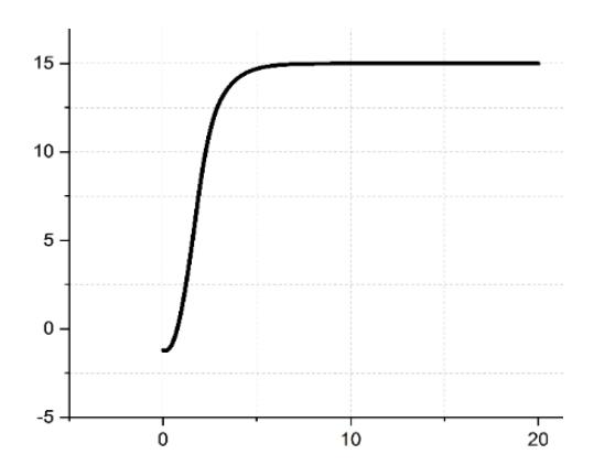
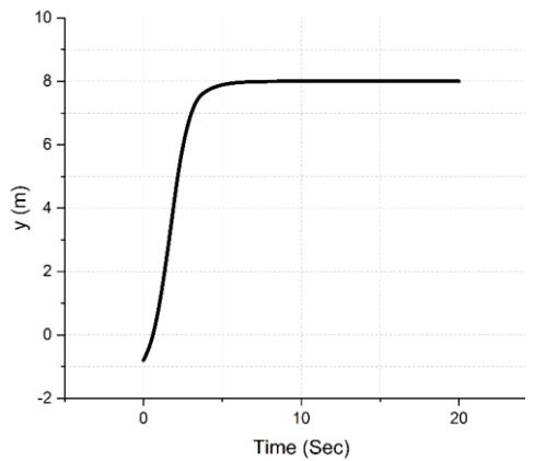
Figure 4 Fixed-Point position response curve. Figure 5 Fixed-Point position response curve.
Fixed-Point Flight Simulation
The tracking targets in the fixed-point flight simulation are 1 = 15, 1 = 8, 1 = 5, and 1=1. Figures 4 to 9 show the simulation results of the UAV's fixed-point flying scenario. These results demonstrate how the proposed approach may improve the system's performance while tracking trajectories.
Figures 4, 5, and 6 show the position tracking performance of the , , and coordinates, respectively. The roll angle response about the -axis is shown in Figure 7. The yaw and pitch are shown in 9 and 8, respectively. Moreover, for the case of a fixed-point trajectory, the sliding surfaces are shown in Figure 10. Figure 11 illustrates the control demand to achieve the closed-loop response. The chattering problem is not as severe as illustrated in the figure because of the relatively acceptable amplitudes of the spikes.
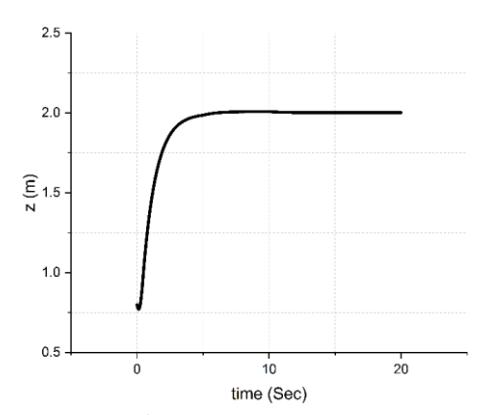
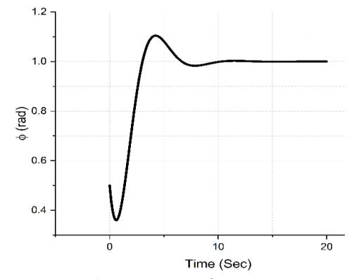
Figure 6 Fixed-Point position response curve. Figure 7 Fixed-Point position response curve.
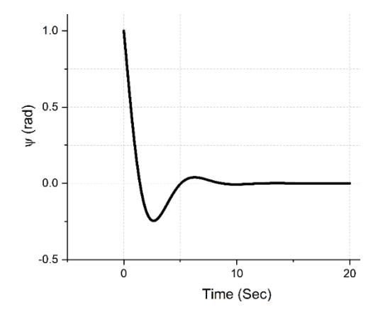
Figure 8 Fixed-Point position response curve. Figure 9 Fixed-Point position response curve.
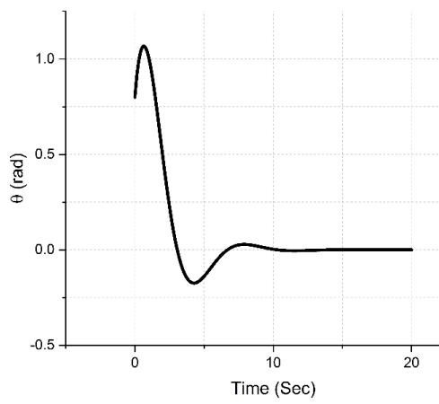
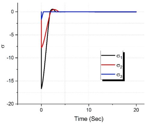
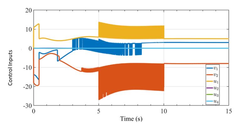
Figure 10 Sliding Surfaces for Fixed-Point tracking. Figure 11 Control inputs for Fixed-Point tracking.
The results demonstrate that the UAV system successfully converges to the desired target values within a finite time. Notably, the proposed control strategy significantly enhances the convergence speed and tracking accuracy, as evidenced by the rapid stabilization of the system's states. This highlights the robustness and efficiency of the proposed method in achieving stable fixed-point flight for UAVs.
Take-off Flight Simulation
In the take-off flight, the tracking target is set to 1 = 0, 1 = 0, 1 = ℎ [ ](ℎ is the height of each step, is the duration of each step) and 1 = 0. These results demonstrate how the proposed approach can enhance the system's trajectory tracking performance. Figures 12, 13, and 14 show the , , and position tracking, respectively. The roll angle dynamics are shown in Figure 15, while Figures 16 and 17 illustrate the yaw and pitch angles. The corresponding sliding surfaces and control inputs are displayed in Figures 18 and 19, respectively.
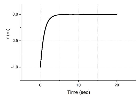
Figure 12Take-off position response curve. Figure 13Take-off position response curve.
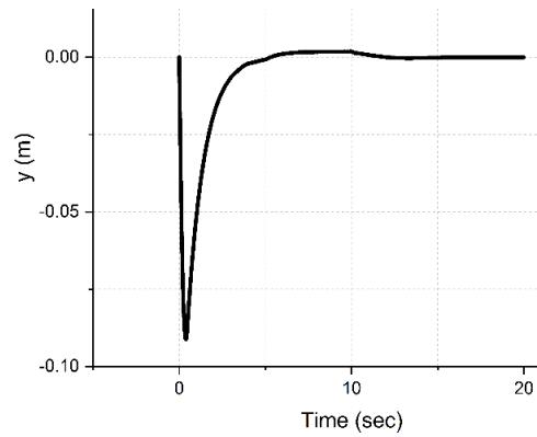
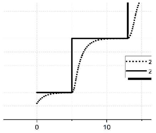
Figure 14Take-off position response curve. Figure 15Take-off Euler angle response curve.
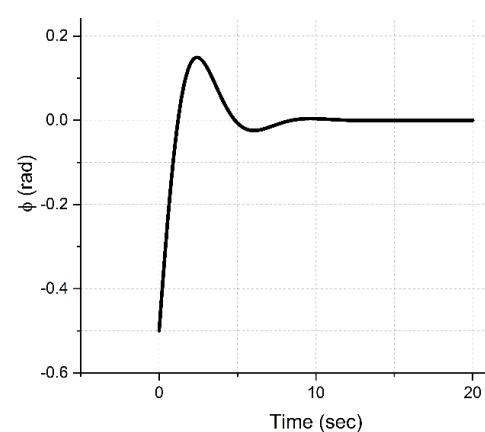
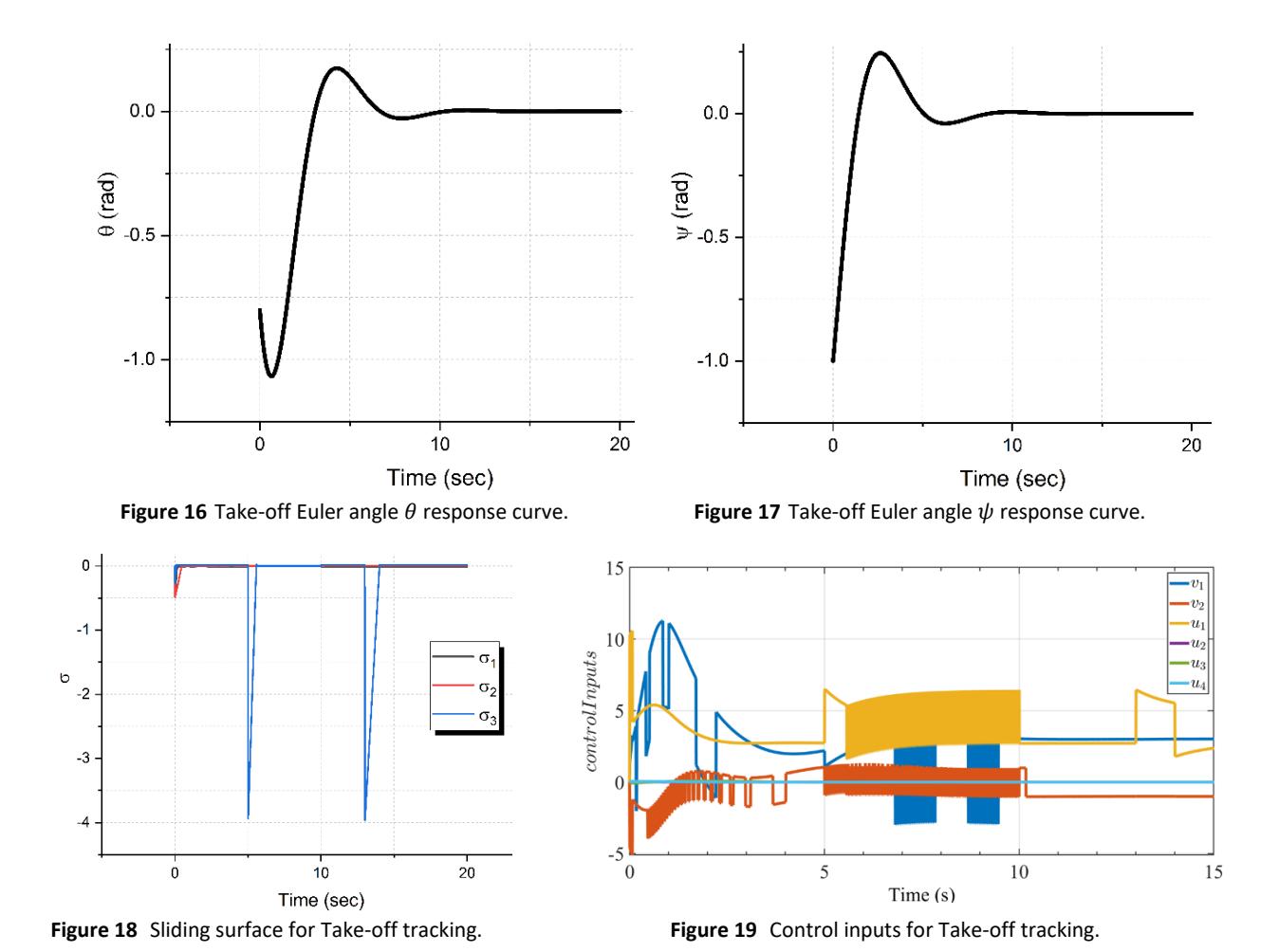
As illustrated in Figures 12 to 19, the simulation data reveal that the UAV system achieves the desired take-off trajectory with high precision and minimal overshoot. The proposed control strategy ensures smooth transitions between steps, as indicated by the consistent tracking performance across all axes. These results underscore the method's effectiveness in handling dynamic flight scenarios, such as take-off, with enhanced stability and convergence.
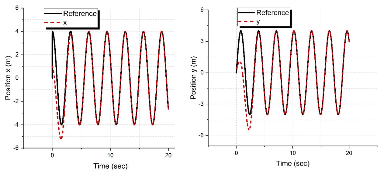
Figure 20 Spiral Trajectory position response curve. Figure 21 Spiral Trajectory position response curve.
Spiral Curve Tracking Simulation
Spiral ascent is a common flight mode of UAVs. This section assumes that the expected trajectory of quadrotor UAVs is a spiral ascent curve, and the desired trajectory is designed as 1 = 5(2), 1 = 3(2), 1 = .4 and 1 = 0.2. The results of this section demonstrate how the proposed approach can enhance the system's performance in tracking trajectories. The simulation results, illustrated in Figures 20 to 28, demonstrate the UAV's tracking performance under this complex trajectory. Figures 20, 21, and 22 show the position tracking along , , and axes, respectively. The roll angle response is shown in Figure 24, while the pitch and yaw responses are shown in Figures 25 and 26, respectively. The sliding surfaces and controller inputs for the spiral trajectory are shown in Figures 27 and 28, respectively.
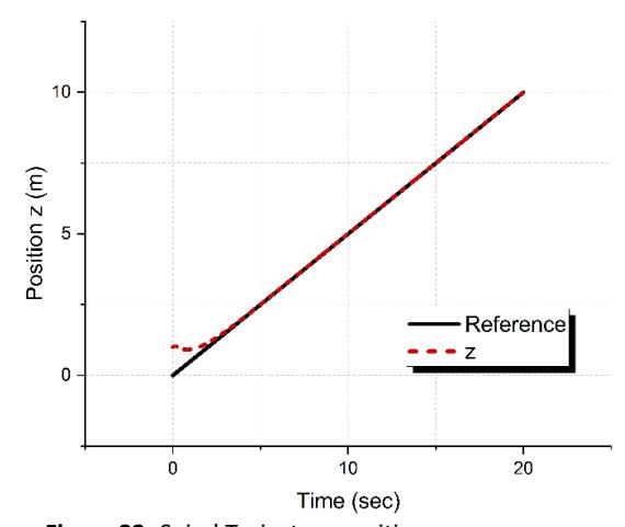
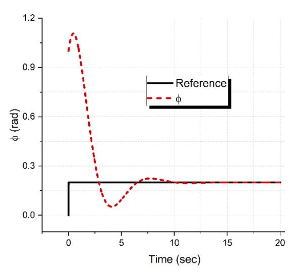
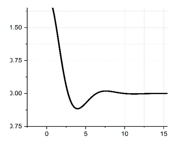
Figure 26 Spiral Trajectory angle response. Figure 27 Sliding Surfaces for Spiral Trajectory tracking.
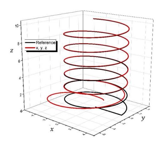
Figure 22 Spiral Trajectory position response. Figure 23 Spiral trajectory tracking diagram.

Figure 24 Spiral Trajectory Euler angle response. Figure 25 Spiral Trajectory Euler angle response.
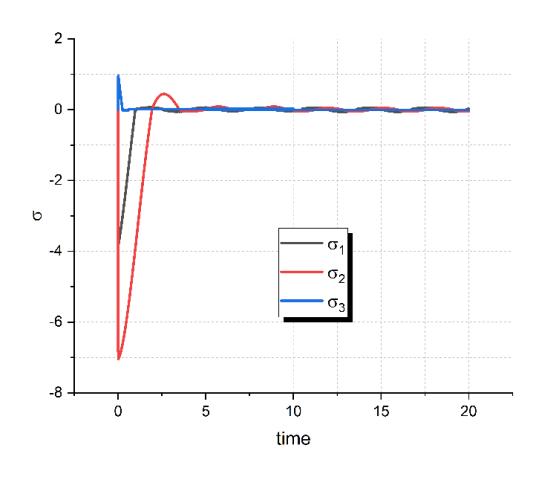
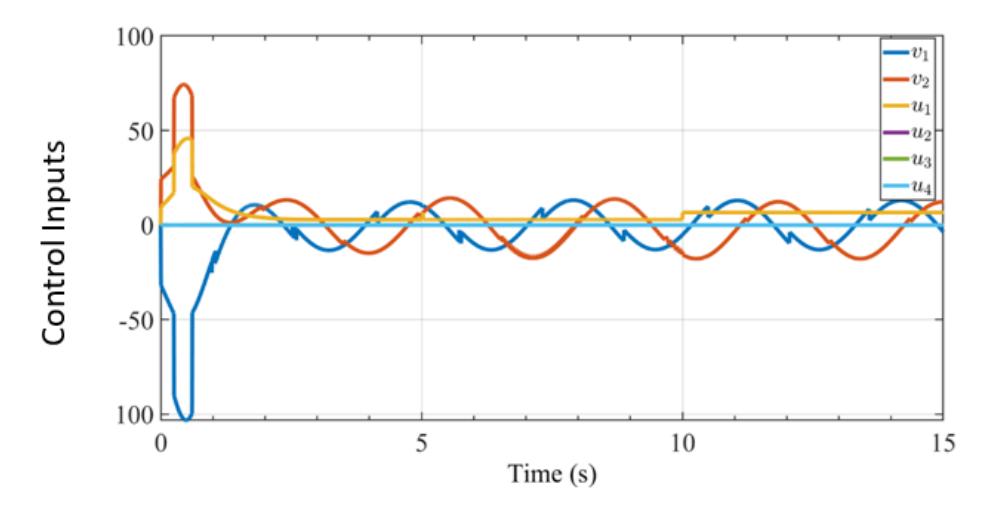
Figure 28 Control input for spiral trajectory.
As illustrated in Figures 20 to 28, the results indicate that the UAV system successfully tracks the spiral ascent trajectory with high accuracy and minimal deviation. The proposed control strategy exhibits excellent performance in handling the nonlinearities and coupling effects inherent in spiral flight, as evidenced by the smooth and consistent tracking across all states. This further validates the method's applicability to complex flight scenarios, ensuring robust and stable operation.
Discussion
The simulation results presented in the previous section clearly highlight the effectiveness and robustness of the proposed control strategy in handling numerous trajectory-tracking missions under different operating envelopes. In the fixed-point scenario, the closed-loop system showed rapid convergence to the desired values with minimal overshoot and chattering. In fact, these measures can be further optimized using advanced algorithms for tuning the controller's gains.
In the take-off maneuver, the closed-loop system demonstrated smooth tracking and transition between steps, which is crucial for safe vertical ascents. Despite the continuities within the steps in the target altitude, the closed-loop system was able to maintain high tracking performance, which reflects the controller's adaptability even in the presence of control input spikes.
For a more challenging nonlinear and coupled dynamics associated with the spiral trajectory tracking maneuver, the proposed controller enabled the UAV to successfully track the 3D spiral trajectory with minimal tracking steady-state error. This behavior proves the controller's ability to handle intricate trajectories in nonlinear regimes effectively.
The proposed control methodology offers several significant advantages over existing techniques, particularly in terms of robustness and comprehensive trajectory tracking. First, while many existing studies neglect external disturbances, the robustness of the proposed method has been rigorously validated. Extensive simulations have been conducted to demonstrate its effectiveness in the presence of external disturbances for various missions, including fixed-point hovering, takeoff, and spiral trajectory tracking. This comprehensive verification is a key strength of the current work, as it confirms the controller's ability to maintain stable and accurate performance under challenging conditions.
Furthermore, the proposed approach addresses several limitations observed in prior research. For instance, the work presented in (Kotch et al., 2019) and (Masse et al., 2018) primarily focuses on applying advanced control techniques like deep reinforcement learning, LQR, and H∞ to attitude control only. Similarly, reference (Polvara et al., 2018) apply a deep reinforcement learning technique exclusively to the specific task of landing control. This work, in contrast, provides a unified solution for full quadcopter trajectory tracking, encompassing position and attitude control simultaneously.
A direct performance comparison with a traditional method, such as the PID controller in (Bayisa and Li, 2019), further highlights the superiority of the proposed controller. The results in (Bayisa and Li, 2019) show a settling time of 5.5 seconds with an overshoot of 3-5% for position tracking. The proposed controller achieves a significantly faster settling time of 3.5 seconds and demonstrates zero overshoot, which indicates a more stable and efficient response.
Finally, when compared to the nonlinear control method in (Abdulkareem et al., 2022), the controller demonstrates superior performance in complex maneuvers. The spiral trajectory tracking presented in (Abdulkareem et al., 2022) lacks the precision and accuracy achieved by the proposed method, which successfully tracks the complex path with minimal error. This confirms the enhanced capability of the current controller for intricate and dynamic tasks.
Conclusion
This paper presented a nonlinear hybrid control strategy for addressing the challenges of low tracking accuracy in attitude and position control associated with the quadrotor UAVs. By integrating adaptive sliding mode control with Lyapunov theory, the proposed method effectively enhances trajectory tracking performance. While improving robustness and flexibility in the presence of external disturbances, the Lyapunov stability theory was utilized to rigorously analyze the stability of the control system, and the results confirmed that the proposed controller ensures system stability under various operating conditions. Extensive simulation tests demonstrated the effectiveness and feasibility of the developed control approach. The simulation results revealed that the proposed method significantly improves tracking accuracy for both attitude and position control, outperforming conventional controllers in terms of convergence speed and precision. In fact, the ability to quickly and accurately track desired trajectories, even in the presence of uncertainties, makes this approach a robust and reliable solution for complex UAV applications. Furthermore, the hybrid control strategy demonstrated strong adaptability, making it suitable for diverse operational scenarios. It provides a systematic paradigm to handle nonlinearities and disturbances while simultaneously maintaining high performance. This makes the proposed method a valuable contribution to the field of UAV control, with potential applications in surveillance, delivery, and other advanced aerial operations. Overall, the proposed nonlinear hybrid control strategy proves to be an effective tool for improving the performance of quadrotor UAVs, ensuring precise trajectory tracking, enhanced robustness, and stability, making it a promising technique for real-world UAV missions. Finally, to capture a more realistic physical representation of external disturbances, a future extension of the current work is to consider more realistic time-varying disturbance models, such as Dryden gusts or stochastic/harmonic models, for improved performance evaluation of the proposed controller. Additionally, to examine the proposed controller's real-world applicability, this work will be extended to incorporate hardware-in-the-loop testing for realtime, practical validation.
Compliance with ethics guidelines
The authors declare they have no conflict of interest or financial conflicts to disclose.
This article contains no studies with human or animal subjects performed by the authors.