
Introduction
Acrylonitrile is a widely used volatile organic compound (VOC) in the petrochemical industry, primarily as a raw material for synthetic fibers, plastics, and rubber production. It does not occur naturally and is mainly emitted from chemical production processes, with over 95% of industrial emissions coming from its use in polymer manufacturing (Long et al., 2002). Acrylonitrile is classified as a high-priority substance under the Toxic Substances Control Act (TSCA) (USEPA, 2016) due to its extensive industrial applications and high production volumes. According to the U.S. Environmental Protection Agency (USEPA, 2024), annual U.S. production has consistently exceeded 1 billion pounds (approximately 450,000 metric tons) since 1986, underscoring its role in the petrochemical and polymer industries (USEPA, 2024). In Thailand, acrylonitrile is primarily imported for industrial use, with import volumes ranging from 9,502 to 25,969 metric tons between 2016 and 2020, according to the Department of Industrial Works. Once released, acrylonitrile disperses into air and water, undergoing atmospheric degradation with a half-life of 55 to 96 hours, while its persistence in aquatic and soil environments can be significantly longer depending on local conditions. Due to its high volatility and hazardous properties, emissions from acrylonitrile storage tanks pose considerable environmental and health risks (Ministry of Public Health, 2012), particularly in industrial areas with large-scale storage and handling. Among VOC emissions from petrochemical storage, flash emissions also occur when stored liquid rapidly depressurizes (TCEQ, 2012) and are of particular concern because they can release high concentrations of VOCs into the atmosphere.
Rayong Province, Thailand, serves as a major hub for petrochemical industries, where emissions from storage tanks have raised concerns about air quality and public health. These industrial areas often contribute to public health risks through airborne VOCs, which may affect populations residing near petrochemical facilities (Thepanondh et al., 2011).
Copyright by authors ©2026 Published by IRCS - ITB J. Eng. Technol. Sci. Vol. 58, No. 2, 2026, 274-286 ISSN: 2337-5779 DOI: 10.5614/j.eng.technol.sci.2026.58.2.9
Acrylonitrile is classified as a potential human carcinogen by the U.S. Environmental Protection Agency (USEPA), with exposure linked to respiratory problems, neurological disorders, and increased cancer risks (USEPA, 1991). Although regulatory agencies have established air quality standards to limit VOC concentrations, controlling emissions from industrial storage facilities remains challenging. This challenge arises from the dynamic nature of flash emissions and the limitations of current mitigation measures.
This study aims to evaluate flash emissions from an acrylonitrile storage tank and their impact on ambient air quality using mathematical and computational models. The Vasquez-Beggs Equation (VBE) (Vazquez & Beggs, 1980) and TANKS 5.1 model (USEPA, 2024) were applied to estimate flash emissions under different operating conditions, while the AERMOD dispersion model (USEPA, 2017) was used to analyze the spatial distribution of acrylonitrile concentrations in the surrounding environment. By assessing emissions under both uncontrolled and controlled scenarios, this research provides insights into the effectiveness of emission control technologies and proposes strategies to mitigate environmental and health risks associated with acrylonitrile storage.
The findings from this study contribute to a better understanding of acrylonitrile emissions and offer recommendations for improving industrial emission control measures. These insights can assist policymakers, regulatory agencies, and industrial operators in implementing more effective VOC management strategies to ensure environmental sustainability and public health protection. Substantial emission reductions are feasible through rapid identification of the root causes of high emissions and the deployment of more reliable systems, enhancing the effectiveness of existing controls and minimizing the environmental footprint of petrochemical operations (Alvarez et al., 2018).
Materials and Methods
This study assessed flash emissions from acrylonitrile storage tanks using emission modeling and air dispersion simulations. The methodology included: (1) emission estimation using the Vasquez-Beggs Equation (VBE) and TANKS 5.1, (2) air dispersion modeling with AERMOD, and (3) risk assessment at receptor locations.
Study Area and Data Collection
The study was conducted at a petrochemical facility in Rayong Province, Thailand, located in the study area shown in Figure 1, where an acrylonitrile storage tank operates under varying temperature and pressure conditions. Data for the emission estimation were obtained from the facility's operational records, including tank dimensions, liquid properties, vapor pressure, temperature, and pressure. Meteorological data, such as wind speed, wind direction, temperature, and atmospheric stability, were obtained from the Thai Meteorological Department and from Lake Environmental Software.
Map of the study area in Rayong Province, Thailand.
Flash Emission Estimation
The Vasquez-Beggs Equation (VBE) was used to estimate the flash gas-oil ratio (GOR) and flash losses from the acrylonitrile storage tank (API, 2009). This model calculates the volume of gas released per unit of liquid under varying pressure conditions. Site-specific data, including separator pressure, separator temperature, liquid density, and gas molecular weight, were applied to the equation. The VBE is an empirical, steady-state correlation that estimates bulk flash VOC emissions based on temperature, pressure, and API gravity. It does not account for the frequency or duration of intermittent events and may over- or under-estimate emissions depending on operational variability.
TANKS 5.1 Model
The U.S. Environmental Protection Agency's (USEPA) TANKS 5.1 model was used to estimate VOC emissions from the storage tank. This model accounts for standing, working, and breathing losses in addition to flash emissions, based on the tank's configuration and environmental conditions (USEPA, 2006). Inputs included tank dimensions, storage temperature, pressure fluctuations, properties of acrylonitrile, and meteorological parameters (USEPA, 2020).
TANKS has been widely applied in studies quantifying VOC emissions from organic liquid storage facilities. Previous research demonstrated its effectiveness in estimating emissions from fixed-roof crude oil tanks, where working and breathing losses were identified as the primary emission sources. In one study, VOC emissions calculated using TANKS were compared with field measurements, showing a strong correlation with observed values (Koçak, 2022). The study also highlighted that meteorological variations, particularly wind speed and temperature fluctuations, significantly influence the emission rates predicted by the model. Given its reliability in estimating VOC emissions, TANKS 5.1 was selected for this study to provide site-specific assessments of acrylonitrile storage. Where available, site-specific operational parameters, such as tank turnover rate, storage time, and venting frequency, were applied; otherwise, default EPA factors were used. These models were chosen because they align with regulatory guidance and are compatible with the available data.
Air Dispersion Modeling
The American Meteorological Society/U.S. Environmental Protection Agency Regulatory Model (AERMOD) was used to simulate the transport and concentration of acrylonitrile emissions in the surrounding environment. The model incorporated meteorological data, terrain features, and receptor locations to assess dispersion patterns under different operating scenarios. A total of 86 receptor locations were selected for analysis, all classified as sensitive receptors, including schools, hospitals, and residential areas susceptible to air pollution exposure. Emission rates obtained from the VBE and TANKS 5.1 models served as inputs to predict acrylonitrile concentrations. Simulations were conducted for both uncontrolled conditions (without emission control measures) and controlled conditions, assuming 90% emission reduction through technologies such as vapor recovery units.
AERMOD was selected for this study due to its ability to incorporate site-specific meteorological parameters, terrain variations, and emission characteristics, making it a robust tool for predicting ground-level concentrations of hazardous air pollutants. Its effectiveness has been demonstrated in studies of emissions from cement plants and other industrial facilities, where the model successfully simulated pollutants such as sulfur dioxide, mercury, arsenic, and chromium to evaluate compliance with ambient air quality standards (Abdel-Gawad et al., 2022). Dispersion modeling in this study was based on an AERMET-ready WRF dataset (surface and upper air) covering a one-year period from January to December 2022. The dataset had an hourly resolution on a 12-km grid and was generated for the Rayong area (12.65856°N, 101.3127°E; elevation 18.13 m; UTC+0700). These data provided the necessary meteorological inputs wind speed, wind direction, temperature, humidity, pressure, and mixing height—for AERMOD simulations and are consistent with U.S. EPA guidance, which recommends at least one year of representative hourly meteorology.
Risk Assessment
To evaluate the potential health risks associated with acrylonitrile exposure, a risk assessment was conducted following USEPA guidelines (USEPA, 2009). Exposure concentrations at receptor locations were compared against reference exposure limits for both acute and chronic inhalation risks. The hazard quotient (HQ) and cancer risk were calculated to determine potential health impacts on nearby communities and workers.
Risk assessment is crucial for evaluating the long-term health effects of VOC exposure, particularly in industrial areas with significant emissions. Studies have shown that prolonged inhalation of VOCs, even at low concentrations, can cause both acute and chronic health effects and increase cancer risk over time. In regions with dense petrochemical activity, risk assessment is essential for identifying high-exposure populations and informing policy decisions on emission control measures (Malakan et al., 2022).
Sensitivity Analysis
To assess the robustness of the conclusions with respect to control performance, a one-parameter sensitivity analysis was conducted by varying overall control efficiency (η) at 70%, 80%, 90%, and 95%. Because AERMOD is linear in source strength, ground-level concentrations, HQ, and cancer risk scale directly with total emission rate (E). Accordingly, new values were obtained by multiplying the uncontrolled baseline results (SC6) by the factor (1–η), as shown in the equation:
\[C_{\eta} = C_0 \times (1 - \eta) \tag{1}\] where Cη is the concentration, HQ, or risk under control efficiency η, and C0 is the baseline (SC6) value. This approach avoids the need to rerun the dispersion model and allows direct estimation of receptor-level impacts under alternative control efficiencies.
Results
The results of this study focus on: (1) the estimation of flash emissions from an acrylonitrile storage tank, (2) air dispersion modeling of emissions under different scenarios, and (3) the potential health risks associated with exposure to acrylonitrile concentrations in ambient air.
Flash Emissions
Flash emissions were calculated using the Vasquez-Beggs Equation (VBE) under varying pressure and temperature conditions. Under midrange operating conditions, flash emissions were estimated at 12.84 g/s, while peak emissions under high-pressure, low-temperature conditions reached 18.17 g/s. In comparison, breathing and working losses calculated using the TANKS 5.1 model were considerably lower, contributing 0.0986 g/s and 0.2776 g/s, respectively, under uncontrolled conditions, as shown in Table 1.
| Condition | Pressure (psig) | Temperature (°F) | Emission Rate (g/s) |
|---|---|---|---|
| Midrange Operating Condition (MO) | 0.064 | 77 | 15.25 |
| Low-Pressure Low-Temperature Condition (LPLT) | 0.0142 | 50 | 18.02 |
| High-Pressure High-Temperature Condition (HPHT) | 0.1137 | 104 | 12.96 |
| High-Pressure Low-Temperature Condition (HPLT) | 0.1137 | 50 | 18.17 |
| Low-Pressure High-Temperature Condition (LPHT) | 0.0142 | 104 | 12.84 |
Table 1 Flashing losses from the Vasquez-Beggs Equation method.
Comparison of emissions
The comparison of acrylonitrile emissions from flashing losses, breathing losses, and working losses highlights the distinct contributions of each source to the overall emission profile of the storage tank. Flashing losses, resulting from rapid pressure reductions, contribute the largest fraction of total emissions, whereas breathing and working losses, driven by temperature fluctuations and liquid transfer processes, represent smaller but consistent contributions.
To quantify these variations, emissions were categorized under different operating conditions, both with and without control measures. Scenarios included emissions calculated using TANKS 5.1 and the Vasquez-Beggs Equation (VBE), with control equipment operating at 90% efficiency in selected cases. Among the evaluated operational conditions, the Low-Pressure High-Temperature (LPHT) scenario was chosen for assessment because it exhibited the lowest emission rate, ensuring optimal control over emission release. The results emphasize the dominance of flashing emissions under uncontrolled conditions and demonstrate the effectiveness of control technologies in reducing total emissions, as shown in Table 2.
The 90% control efficiency scenario represents advanced VOC abatement systems applicable to petrochemical storage tanks. Relevant technologies include vapor recovery units (VRUs), activated carbon adsorption systems with regeneration, and thermal or regenerative thermal oxidizers. Reported efficiencies for these technologies range between 80–95%, depending on design and operating conditions. A value of 90% was selected to reflect an ambitious yet achievable level of performance, consistent with published ranges and current industrial practice.
The findings indicate that flashing losses, calculated using the Vasquez-Beggs Equation (VBE), were the dominant contributor to total emissions. In the absence of control measures, emissions from flashing losses alone reached 12.84 g/s, far exceeding the combined working and breathing losses across all scenarios. The highest total emissions were observed in Scenario 6 (13.22 g/s), which reflected the sum of all uncontrolled sources.
Conversely, applying 90% control efficiency resulted in substantial emission reductions. Scenario 7, which implemented control measures for all sources, produced the lowest total emissions at 1.322 g/s, representing an 89% decrease compared with the Worst-Case scenario. These results underscore the effectiveness of comprehensive emission control strategies.
A comparison between Scenario 5 (12.88 g/s, with controlled working and breathing losses but uncontrolled flashing losses) and Scenario 7 (1.322 g/s, full control) further highlights the importance of mitigating flashing losses. While working and breathing losses contribute to total emissions, the predominance of flashing losses makes advanced control technologies essential. Integrating effective control systems with reliable modeling approaches will support compliance with environmental standards and significantly reduce the environmental impact of acrylonitrile storage tank operations.
| Scenarios | Conditions | Working Losses (g/s) | Breathing Losses (g/s) | Flashing Losses (g/s) | Total Emissions (g/s) |
|---|---|---|---|---|---|
| SC1 | TANKS 5.1 without control | 0.2776 | 0.0986 | - | 0.3761 |
| SC2 | TANKS 5.1 with 90% control efficiency | 0.0279 | 0.0098 | - | 0.0377 |
| SC3 | Vasquez-Beggs Equation without control | - | - | 12.84 | 12.84 |
| SC4 | Vasquez-Beggs Equation with 90% control efficiency | - | - | 1.284 | 1.284 |
| SC5 | Combined emissions from TANKS 5.1 (with control) and VBE (without control) Combined emissions from | 0.0279 | 0.0098 | 12.84 | 12.88 |
| SC6 | TANKS 5.1 and VBE, both without control | 0.2776 | 0.0986 | 12.84 | 13.22 |
| SC7 | Combined emissions from TANKS 5.1 and VBE, both with 90% control efficiency | 0.0279 | 0.0098 | 1.284 | 1.322 |
Table 2 Emission scenarios and control efficiency comparison.
Air Dispersion Modeling
Dispersion modeling using AERMOD was performed to evaluate the spatial distribution of acrylonitrile emissions from the storage tank under different control scenarios. Emissions from working losses, breathing losses, and flashing losses were incorporated into the model to assess their impact on air quality at receptor locations near the industrial site. Acrylonitrile concentration maps were generated to visualize dispersion patterns. Uncontrolled emissions resulted in the highest concentrations, exceeding 800 μg/m³ (24-hour average) near the source, as shown in the spatial distribution of acrylonitrile concentrations under Scenario 5 in Figure 2 and under Scenario 6 in Figure 3, indicating potential shortterm exposure risks for nearby receptors. Applying 90% control efficiency significantly reduced peak concentrations, as shown in the spatial distribution of acrylonitrile concentrations under Scenario 7 in Figure 4, although localized areas of concern remained where concentrations exceeded applicable air quality guidelines.
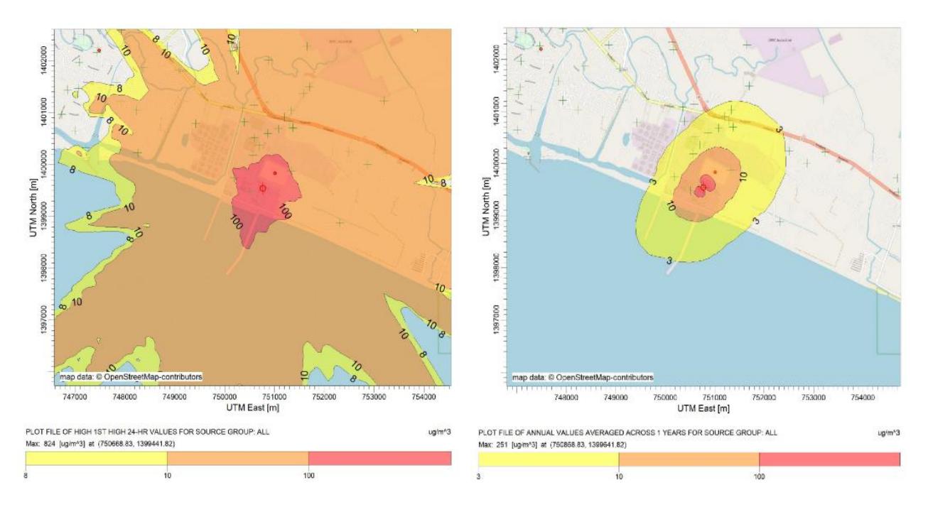
Scenario 5: Acrylonitrile Concentration, 24-Hour Average and Annual Averaging.
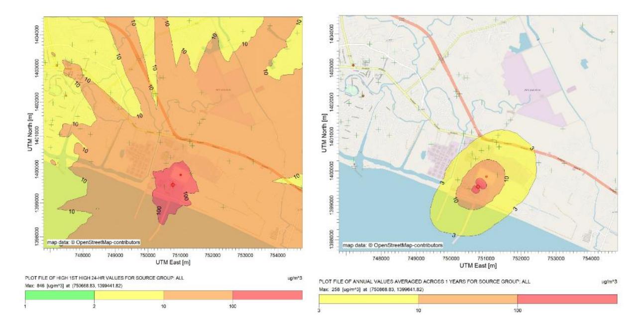
Scenario 6: Acrylonitrile Concentration, 24-Hour Average and Annual Averaging
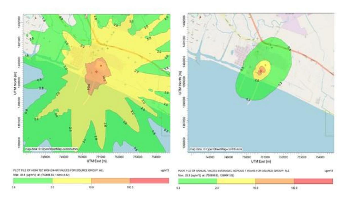
Scenario 7: Acrylonitrile Concentration, 24-Hour Average and Annual Averaging.
Concentration at Receptor Sites
Annual average concentrations at 86 receptor locations, including schools, residential areas, and healthcare facilities, were compared with the USEPA Reference Concentration for Inhalation Exposure (RfC) of 2 μg/m³ for chronic exposure. Under uncontrolled scenarios, annual concentrations exceeded 250 μg/m³, particularly at receptors closest to the emission source. Applying control measures substantially reduced concentrations, with most locations fa lling below 25 μg/m³, demonstrating the effectiveness of emission mitigation strategies. However, despite these reductions, several receptor sites still exceeded the RfC threshold, indicating the need for further optimization of emission control measures. These findings emphasize the dominant contribution of flashing losses to overall VOC concentrations and underscore the importance of advanced emission control technologies to reduce environmental and health risks in industrial areas.
Risk Assessment of Acrylonitrile Emissions
A comprehensive risk assessment of acrylonitrile (ACN) emissions from the storage tank was conducted to evaluate potential health risks at receptor locations under various emission control scenarios. The assessment addressed both non-carcinogenic and carcinogenic risks by examining hazard quotient (HQ) values and cancer risk estimates across selected receptors.
From the 86 identified receptor sites, 9 key receptors were selected for detailed evaluation due to their proximity to the emission source and their annual average ACN concentrations exceeding the Reference Concentration for Inhalation Exposure (RfC) of 2 μg/m³. These receptors, located within a 2-km radius, represent the most impacted areas where exposure risks are expected to be the highest.
Non-carcinogenic risks were assessed using HQ values, where values exceeding 1.0 indicate potential health concerns. Under the Business-As-Usual scenario (SC5), HQ values remained elevated across all selected receptors, particularly at WPKS, ITC, HPB, RPC, WPK, PNUF, RPVC, WPKS2, and TYB. Compared to the Worst-Case scenario (SC6), HQ values increased by 2.6–2.7%, highlighting the impact of uncontrolled emissions. In contrast, under the Best-Case scenario (SC7), HQ values decreased by 89.7%, demonstrating that 90% control efficiency effectively mitigates non-carcinogenic health risks.
Carcinogenic risks showed a similar pattern, with cancer risk values at the selected receptors exceeding the acceptable regulatory thresholds (1.0 × 10⁻⁶) in SC5 and increasing by 2.5–2.8% in SC6. Implementation of SC7 substantially reduced cancer risk levels by 89.7%, although some receptors still exceeded the threshold, indicating that further mitigation measures may be necessary to reduce long-term health risks.
Despite these improvements, flashing losses remained the dominant contributor to elevated risk levels. Unlike continuous emissions from working and breathing losses, flashing losses occur intermittently during acrylonitrile transfer processes, meaning real-world exposure may fluctuate rather than remain consistently high. This suggests that, while modeled risk assessments indicate elevated values, actual long-term exposure levels may be lower than the modeled annual averages.
| HQ | Cancer Risk | ||||||
|---|---|---|---|---|---|---|---|
| Receptor | SC5 | SC6 | SC7 | SC5 | SC6 | SC7 | Distance (km) |
| WPKS | 0.2971 | 0.3049 | 0.0305 | 4.04 × 10⁻⁵ | 4.15 × 10⁻⁵ | 4.15 × 10⁻⁶ | 1.31 |
| ITC | 0.132 | 0.1355 | 0.0135 | 1.79 × 10⁻⁵ | 1.84 × 10⁻⁵ | 1.84 × 10⁻⁶ | 2 |
| HPB | 0.2218 | 0.2277 | 0.0228 | 3.02 × 10⁻⁵ | 3.10 × 10⁻⁵ | 3.10 × 10⁻⁶ | 1 |
| RPC | 0.1907 | 0.1958 | 0.0196 | 2.59 × 10⁻⁵ | 2.66 × 10⁻⁵ | 2.66 × 10⁻⁶ | 1.61 |
| WPK | 0.2997 | 0.3076 | 0.0308 | 4.08 × 10⁻⁵ | 4.18 × 10⁻⁵ | 4.18 × 10⁻⁶ | 1.3 |
| PNUF | 0.1448 | 0.1487 | 0.0149 | 1.97 × 10⁻⁵ | 2.02 × 10⁻⁵ | 2.02 × 10⁻⁶ | 1.87 |
| RPVC | 0.2212 | 0.227 | 0.0227 | 3.01 × 10⁻⁵ | 3.09 × 10⁻⁵ | 3.09 × 10⁻⁶ | 1.43 |
| WPKS2 | 0.2473 | 0.2546 | 0.0255 | 3.36 × 10⁻⁵ | 3.46 × 10⁻⁵ | 3.46 × 10⁻⁶ | 1.39 |
| TYB | 0.3009 | 0.3098 | 0.031 | 4.09 × 10⁻⁵ | 4.21 × 10⁻⁵ | 4.21 × 10⁻⁶ | 1.19 |
| RCPV | 0.0616 | 0.0633 | 0.0063 | 8.38 × 10⁻⁶ | 8.60 × 10⁻⁶ | 8.60 × 10⁻⁷ | 2.47 |
| RKS | 0.0158 | 0.0162 | 0.0016 | 2.15 × 10⁻⁶ | 2.21 × 10⁻⁶ | 2.21 × 10⁻⁷ | 4.28 |
Table 3 Risk assessment and distances of selected receptors sites.
The spatial distribution of risk was further analyzed based on the distance of each receptor from the emission source. As shown in Table 3, receptors closest to the source, such as HPB (1.00 km) and TYB (1.19 km), exhibited highest HQ and cancer risk values, consistent with the expectation that proximity correlates with increased exposure. However, even receptors beyond 2 km, such as ITC (2.00 km), exceeded the RfC limit, indicating that the impact of emissions extends beyond the immediate vicinity of the storage tank.
In contrast, receptors farther from the source, such as RCPV (2.47 km) and RKS (4.28 km), showed substantially lower HQ and cancer risk values, reinforcing that distance is a key factor in exposure reduction. These findings highlight the importance of targeted mitigation efforts within the 2-km high-exposure zone, where populations remain most vulnerable to ACN emissions.
Sensitivity Analysis of Total Emission Rate and Risk Assessment
In addition to the base case scenarios, a sensitivity analysis was conducted to evaluate the robustness of results under different control efficiencies. Given the linearity of the dispersion model with respect to source strength, emission rates, ground-level concentrations, hazard quotients (HQ), and cancer risk values were scaled directly according to the assumed efficiency. Efficiencies of 70%, 80%, 90%, and 95% were examined to assess how emission reductions translate into changes in exposure and risk at receptor locations. Five representative receptors (WPKS, TYB, HPB, WPK, and RPC) were selected to illustrate the results, as these sites exhibited the highest risks in the base scenario. Other receptors showed the same proportional reductions and are therefore not presented in detail.
| Table 4 | Sensitivity analysis of total emission rate under different control efficiencies |
|---|
| Control efficiency (η) | Total emission rate (g/s) | ||
|---|---|---|---|
| 0% (uncontrolled, SC6) * | 13.22 | ||
| 70% | 3.97 | ||
| 80% | 2.64 | ||
| 90% (SC7) | 1.32 | ||
| 95% | 0.66 | ||
Table 5 Sensitivity of HQ values at selected receptors under different control efficiencies
| Receptor | HQ (SC6, η=0%) | 70% | 80% | 90% | 95% |
|---|---|---|---|---|---|
| WPKS | 0.3049 | 0.0915 | 0.061 | 0.0305 | 0.0152 |
| TYB | 0.3098 | 0.0929 | 0.062 | 0.031 | 0.0155 |
| HPB | 0.2277 | 0.0683 | 0.0455 | 0.0228 | 0.0114 |
| WPK | 0.3076 | 0.0923 | 0.0615 | 0.0308 | 0.0154 |
| RPC | 0.1958 | 0.0587 | 0.0392 | 0.0196 | 0.0098 |
| Receptor | HQ (SC6, η=0%) | 70% | 80% | 90% | 95% |
|---|---|---|---|---|---|
| WPKS | 4.15×10⁻⁵ | 1.25×10⁻⁵ | 8.30×10⁻⁶ | 4.15×10⁻⁶ | 2.08×10⁻⁶ |
| TYB | 4.21×10⁻⁵ | 1.26×10⁻⁵ | 8.42×10⁻⁶ | 4.21×10⁻⁶ | 2.11×10⁻⁶ |
| HPB | 3.10×10⁻⁵ | 9.30×10⁻⁶ | 6.20×10⁻⁶ | 3.10×10⁻⁶ | 1.55×10⁻⁶ |
| WPK | 4.18×10⁻⁵ | 1.25×10⁻⁵ | 8.36×10⁻⁶ | 4.18×10⁻⁶ | 2.09×10⁻⁶ |
| RPC | 2.66×10⁻⁵ | 7.98×10⁻⁶ | 5.32×10⁻⁶ | 2.66×10⁻⁶ | 1.33×10⁻⁶ |
Table 6 Sensitivity of cancer risk values at selected receptors under different control efficiencies
The sensitivity analysis (Tables 4–6) shows that total emissions decrease proportionally with increasing control efficiency, from 13.22 g/s in the uncontrolled case (SC6) to 0.66 g/s at 95% control. Receptor-level HQ and cancer risk values also decrease accordingly, with high-risk receptors such as WPKS and TYB approaching or falling below the benchmark of 1×10⁻⁶ risk at 95% control. These results confirm that the overall conclusions are robust across the practical efficiency range of 70–95%.
Discussion
The results of this study highlight the significant impact of acrylonitrile (ACN) emissions from storage tanks on ambient air quality and public health. Emission estimation demonstrated that flashing losses are primarily influenced by pressure and temperature conditions in the separator system. These parameters determine the extent of vaporization during rapid depressurization of liquid acrylonitrile (Qin et al., 2023). Among the different emission sources, flashing losses contribute the largest proportion of total emissions, exceeding those from working and breathing losses. Under uncontrolled conditions, peak flash emissions reached 18.17 g/s, whereas breathing and working losses contributed only 0.0986 g/s and 0.2776 g/s, respectively. These findings reinforce the dominant role of flash emissions in determining total VOC concentrations and emphasize the need for targeted emission control strategies.
Recent studies indicate that VOC composition and volatility significantly influence atmospheric persistence and transport. Acrylonitrile exhibits relatively high reactivity due to its short atmospheric half-life. The interaction of ACN with atmospheric oxidants, such as hydroxyl radicals, leads to the formation of secondary air pollutants, including formaldehyde and hydrogen cyanide, which contribute to broader environmental impacts (Cole et al., 2008). These degradation pathways must be considered when assessing long-term exposure risks and potential secondary pollution effects.
The dispersion modeling results indicated that ACN concentrations exceeded 800 μg/m³ (24-hour exposure) in the vicinity of the emission source, posing short-term exposure risks. The highest 24-hour average concentrations were observed in uncontrolled scenarios, particularly at locations within a 2-km radius. Even with the implementation of a 90% control efficiency system, localized exceedances still surpassed regulatory thresholds, highlighting the need for further mitigation measures.
The risk assessment provided further insights into the health implications of ACN exposure. Among the 86 receptor sites analyzed, nine key receptors were identified as high-risk locations due to their proximity to the emission source and annual average ACN concentrations exceeding the Reference Concentration for Inhalation Exposure (RfC) of 2 μg/m³. Hazard quotient (HQ) values in the Business-As-Usual (SC5) scenario ranged from 0.1320 to 0.3009, indicating potential non-cancer health risks, while cancer risk values exceeded acceptable regulatory limits (1 × 10⁻⁶). Under the Worst-Case scenario (SC6), HQ and cancer risk values increased by 2.5–2.8%, demonstrating the impact of uncontrolled emissions. The implementation of SC7 (Best-Case scenario) significantly reduced health risks by approximately 89.7%, yet certain receptors still exceeded acceptable thresholds. This suggests that while control measures effectively reduce risk, additional mitigation strategies may be necessary. These include enhanced control technologies such as vapor recovery systems, thermal oxidizers, activated carbon adsorbers, cryogenic condensation systems, or optimized separator operations.
Furthermore, research has emphasized the importance of refining separator operations to minimize flashing losses, particularly in volatile chemical storage facilities. Optimizing pressure regulation and temperature control during ACN transfer processes has been identified as a key strategy for reducing peak flash emissions, thereby mitigating overall risk to nearby communities.
A key observation from this study is that intermittent flashing losses drive both emission concentrations and health risks, unlike continuous emissions from working and breathing losses. This intermittent nature suggests that while modeled risk assessments indicate elevated annual values, actual exposure may fluctuate over time, potentially resulting in lower real-world risk.
These findings align with previous studies on industrial VOC emissions, reinforcing the importance of adopting stringent emission control measures. While the 90% control efficiency applied in SC7 demonstrated a substantial reduction in emissions and associated risks, the persistence of localized exceedances suggests that site-specific mitigation approaches should be explored. Future research should focus on real-time monitoring techniques and advanced emission capture technologies. Additionally, improved risk assessment methodologies are needed to better characterize and mitigate exposure risks in industrial settings. Advancements in real-time VOC monitoring have demonstrated the potential for enhanced detection of intermittent emissions, allowing for improved regulatory compliance and adaptive mitigation strategies. High-frequency monitoring systems integrated with predictive modeling could provide a more dynamic understanding of emission trends, supporting proactive risk management in high-risk industrial areas. Additionally, data collection on the frequency of flashing events should include operational parameters such as pressure and temperature during each cycle. The future implementation of leak detection technologies or advanced monitoring systems could enhance real-time tracking of acrylonitrile releases and provide early warnings for excessive emissions. Such information would provide valuable insights into the variability of emissions over time and support more accurate risk assessments and control strategies in subsequent studies.
This study has several methodological limitations that should be noted. Although flashing losses occur intermittently during liquid transfer or depressurization events, the Vasquez–Beggs Equation (VBE) was developed to estimate flash emissions from storage tanks under specified operating conditions. By design, VBE provides bulk emission rates under steady-state inputs and does not explicitly capture the frequency or duration of individual events. In this study, VBE outputs were therefore applied as conservative steady inputs to dispersion modeling, consistent with standard practice. To improve representativeness, future assessments should incorporate operational records, such as tank turnover rate and venting time, allowing conversion of VBE results into time-weighted average emissions.
In the absence of site-specific measurements of acrylonitrile (ACN) flash emissions, a qualitative comparison with published field data was included to enhance credibility. Johnson et al. (2022) conducted a measurement campaign across 15 natural gas production sites, quantifying 224 emission sources, including 153 storage tanks. Despite the presence of control devices, tanks contributed about 25% of site emissions, and capture efficiencies ranged from 63– 92%. This efficiency range closely aligns with the 70–95% control scenarios applied in the present study, supporting the plausibility of the assumptions used. Moreover, the uncontrolled flash emission rates estimated here (12–18 g/s) are consistent with the order of magnitude of VOC losses reported in petrochemical tank studies. Although direct validation was not possible, consistency with published measurements strengthens confidence in the representativeness of the VBE and TANKS 5.1 estimates.
While the SC7 scenario with 90% control efficiency reduced overall risks by nearly 90% at all receptors, site-specific mitigation measures were not explicitly analyzed. High-risk receptors such as WPKS and TYB highlight the potential need for targeted actions to further reduce localized exposures. Possible approaches include local shielding or operational adjustments (e.g., scheduling transfer or venting during low-occupancy periods). Although beyond the scope of this study, such receptor-focused strategies represent important directions for future research and practical implementation, linking risk assessment outcomes with actionable site-level interventions.
Finally, additional pollutants, economic feasibility, and the policy context should be considered. Formaldehyde and hydrogen cyanide are known degradation products of ACN and may pose additional health risks. These secondary pollutants were not explicitly modeled here, as AERMOD is limited to the dispersion of primary emissions without chemical transformation. Future studies should employ chemical transport or photochemical models to evaluate secondary formation and fate for a more comprehensive risk assessment. In addition to conventional technologies such as VRUs, activated carbon, and thermal oxidizers, recent advancements in VOC control include plasma-catalytic systems, catalytic ozonation, and novel sorbents such as MOFs (Chang et al., 2022; Mu et al., 2022; Liu et al., 2022; Li, 2024). While still emerging, these approaches may provide higher selectivity and efficiency for VOC capture and destruction in future applications. Beyond technical performance, economic and policy considerations are critical for practical implementation. Vapor recovery units, activated carbon adsorption, and thermal oxidizers represent proven technologies, but capital and operational costs can be substantial. VRUs offer partial cost recovery through solvent reuse, whereas oxidizers impose higher ongoing expenses. Future work should therefore evaluate cost–benefit tradeoffs to support decision-making. From a regulatory standpoint, Thailand currently regulates VOC emissions under the Factory Act and ministerial notifications, but no ambient standard exists specifically for ACN. Our results indicate that uncontrolled emissions can exceed international reference values, and even with 90% control efficiency, certain receptor risks remain above USEPA RfC. These findings highlight the need for stronger site-level control measures within Thailand's framework. At the regional level, ASEAN has yet to establish a binding directive on VOC control, although cooperative mechanisms such as the ASEAN Agreement on Transboundary Haze Pollution and ozone precursor initiatives provide potential entry points. The present study thus offers evidence to support both national and regional
dialogues on strengthening VOC management policies and integrating advanced control technologies into regulatory frameworks.
Conclusion
Acrylonitrile (ACN) emissions from storage tanks were predominantly driven by flashing losses, which contributed significantly higher emission rates than working and breathing losses. In the Worst-Case scenario (SC6), total emissions reached 13.22 g/s, with flashing losses alone contributing 12.84 g/s, far exceeding emissions from other sources. In contrast, the Best-Case scenario (SC7), with 90% control efficiency applied, reduced total emissions to 1.322 g/s, an 89.7% reduction.
Dispersion modeling indicated that under uncontrolled conditions, 24-hour peak ACN concentrations exceeded 800 μg/m³ near the source, substantially surpassing the Reference Concentration for Chronic Inhalation Exposure (RfC) of 2 μg/m³. Annual average concentrations at key receptor sites, such as Wat Pluak Khet School (WPKS) and the 10-Year Building (TYB), also exceeded regulatory limits, with values reaching 4.87 μg/m³ and 4.95 μg/m³, respectively. Even with 90% control, localized exceedances still surpassed the RfC threshold, highlighting the need for additional mitigation measures.
Risk assessment results confirmed that Hazard Quotient (HQ) values in SC5 (business-as-usual scenario) ranged from 0.132 to 0.3009, while cancer risk values were between 1.79 × 10⁻⁵ and 4.09 × 10⁻⁵, exceeding the acceptable threshold of 1.0 × 10⁻⁶. Compared to SC6 (worst case), HQ and cancer risk increased by 2.6–2.7%, while in SC7 (best case), these values decreased by nearly 89.7%, demonstrating the effectiveness of emission controls. However, several receptor sites within a 2-kilometer radius still exhibited risk levels above regulatory thresholds, indicating persistent localized exposure concerns.
To further minimize emissions and associated health risks, additional mitigation strategies should be implemented, including advanced control technologies, optimized separator operations, and real-time emission monitoring systems. While the modeling results provide critical insights into acrylonitrile dispersion and exposure risks, future studies should incorporate real-time monitoring data to validate modeled estimates and improve exposure assessment accuracy. Technologies such as FTIR (Fourier Transform Infrared Spectroscopy), FID (Flame Ionisation Detection), and UAV-based gas sensors offer opportunities for continuous or near-continuous detection of acrylonitrile releases. Continuous monitoring of ACN tanks is technically feasible using high-sensitivity FTIR or FID systems, although practical challenges, including cost, calibration, and safety requirements, remain. In the near term, periodic monitoring with UAVs or fixed detectors may represent a cost-effective solution, while longer-term adoption of continuous systems could further strengthen early detection and risk management. Additionally, future research should focus on refining risk assessment methodologies, improving emission control techniques, and collecting detailed operational data, such as pressure and temperature fluctuations during each transfer cycle, to enhance both the accuracy of emission estimates and regulatory compliance while mitigating long-term environmental and health impacts.
Acknowledgement
The authors would like to acknowledge the support of IRPC Company for providing access to operational data and technical assistance.
Compliance with ethics guidelines
The authors declare they have no conflict of interest or financial conflicts to disclose.
This article contains no studies with human or animal subjects performed by the authors.