
Introduction
Single-phase induction motors (SPIM) are crucial in domestic and industrial applications due to their low cost and robust construction (Hussain & Usman, 2021). However, precise speed control remains difficult, this is due to nonlinearities, parameter variation, and measurement constraints in low-cost systems (Fikireselam & Zerihun, 2022). To address these challenges and avoid the use of physical speed sensors, sensorless strategies are preferred. These approaches combine estimation and intelligent control.
Sensorless speed control has attracted significant interest recently, as it eliminates the need for physical speed sensors. This reduction lowers costs and enhances reliability (Irianto, Murdianto, Sunarno, Proboningtyas, & Dewinta, April 2021). Conventional PID controllers are simple and widely adopted, but their performance deteriorates under nonlinearity and changing loads. To address this, fuzzy logic controllers (FLC) have been introduced to improve adaptability. However, using FLC alone can result in limited steady-state accuracy. As a result, hybrid schemes that combine estimation and intelligent control have emerged to address these limitations. Prior studies have shown that fuzzy-based PID approaches enhance transient response and error metrics in induction machines, while MRAS-based estimators provide reliable rotor-speed estimates for sensorless control (Mohamed, El-Sehiemy, & A, 2019).
This paper explored integrating the Model Reference Adaptive System (MRAS) and the Fuzzy-PID-PID regulator as an advanced approach for sensorless speed regulation in single-phase induction motors. This method presents a promising avenue for enhanced efficiency and accuracy of speed control (Sujeet, Manish, & Anand, July 2022). The MRAS scheme has been used for rotor resistance and speed estimation. By measuring stator voltages and currents, one can estimate rotor speed and resistance simultaneously, using an adjustable model in the stationary stator reference frame and a
Copyright by authors ©2026 Published by IRCS - ITB J. Eng. Technol. Sci. Vol. 58, No. 2, 2026, 379-396
reference model (Zorgani, Hajji, Koubaa, & Boussak, 2023). MRAS adapts to varying operating conditions, making it attractive choice for dynamic systems like induction motors. Incorporating MRAS into the control scheme helps the system adapt to changes in motor parameters and ensures robust, reliable speed control.
A Fuzzy-PID regulator enhances transient response and maintains stable speed regulation across different voltages. It plays a crucial role in fast and accurate speed estimation (Hamdi, Hammoudi, & Betka, 2023). By refining traditional PID control with fuzzy logic, this approach improves adaptability and compensates for nonlinearities in motor behaviour. Changing the speed of induction motors requires controlling the magnitude of voltage and frequency. Voltage/Frequency (V/F) control requires only a few components for implementation (Mohamed, El-Sehiemy, & A, 2019); (Mugheri & Keerio, 2021) However, the Fuzzy-PID control method struggles with high dynamic performance, as well as extremely low operations and applications that need direct control of motor torque rather than frequency (Tejeshree & S, August 2020). Incorporating fuzzy logic overcomes these challenges by enabling intelligent decisions based on error signals and their rate of change.
Appliances use fuzzy controllers because they provide a short rise time, avoid unwanted overshoot, and produce low steady-state error, leading to fewer oscillations (Irianto, Murdianto, Sunarno, Proboningtyas, & Dewinta, April 2021). Because fuzzy controllers can handle non-linear, unsettled systems without a mathematical model, complex systems require many rules for implementation. This makes them overwhelming and tedious (Bhinav & Deshpande, 2021). Fuzzy-PI control of an induction motor operates at speed error to maximize its advantage. The motor's speed is regulated by a Fuzzy logic controller. It uses predetermined rules that govern the fuzzy controller inputs and outputs (Md Shah & Paliwal, May 2018). The fuzzy controller receives two inputs: the error and the change in the error signal. Fuzzy-PID controllers use fuzzy logic to refine traditional PID parameters. They employ a set of optimization rules.
Integration of a Fuzzy-PID regulator introduced a level of intelligent decision-making to the control system. Fuzzy logic enables the integration of human-like reasoning into controllers, allowing them to handle uncertainties and accommodate the non-linearities inherent in the motor's behaviour. The combination of MRAS and Fuzzy-PID created a synergistic effect, where adaptability and intelligent control mechanisms work in concert to improve the sensorless speed control system's overall performance, aiming to construct a precise, reliable, and economical control system which contributes significantly to the advancement in speed control stabilization in induction motor. This work proposes a cascade integration of MRAS with a Fuzzy-PID regulator for sensorless SPIM speed control. Unlike conventional MRAS– PID or Fuzzy–PID structures, the proposed MRAS–Fuzzy-PID controller forms an adaptive hybrid model capable of realtime self-tuning under varying load conditions. This integration for single-phase motor drives represents a new approach that enhances speed estimation accuracy, robustness, and dynamic performance (Manoj, May 2016), (Soni, Khemariya, & Singh, July 2022).
Materials and Methods
Mathematical Model of a Sensorless Single-Phase Induction Motor
The sensorless speed control mathematical model of SPIM is essential for designing induction motor speed controls. It describes both electrical and mechanical differential equations. The stator and rotor voltages formulae, along with equations for flux and torque, are necessary for SPIM operation. The single-phase induction machine consists of a primary and an auxiliary stator winding, and a squirrel-cage rotor. The auxiliary winding usually operates only at startup. For low-power applications, it can stay on during operation to enhance performance (MathWorks). Figures 1 and 2 illustrate the analogous d- and q-axis circuits for the primary and secondary windings.
q-axis (Main winding).
Figure 2 d-axis (Auxiliary winding).
The fundamental voltage equations for stator and rotor, as well as the equations of torque and flow, were derived in order to create a mathematical model of an SPIM. The following voltage equations for the model using Kirchhoff's Voltage Law (Elattar & Amer, 2018):
Stator (d–q) equations \[V_{qs}=R_s i_{qs}+\frac{d\phi_{qs}}{dt}\] (1)
\[V_{ds} = R_a i_{ds} + \frac{d\phi_{ds}}{dt} \tag{2}\]
Rotor (d–q) equations \[V_{qr}=0=R_r'i_{qr}'+\frac{d\phi_{qr}'}{dt}-\frac{1}{K}\omega_r\phi_{qr}'\]
\[V_{dr} = 0 = K^2 R_r' i_{dr}' + \frac{d\phi_{dr}'}{dt} + K\omega_r \phi_{dr}'\] (4)
Then the flux equations were also derived as follows.
Flux linkages \[\phi_{qs} = (L_{ls} + L_{ms})i_{qs} + L_{ms}i'_{qr}\] (5)
\[\phi_{ds} = (L_{la} + K^2 L_{ms}) i_{ds} + K^2 L_{ms} i'_{dr}\] (6)
\[\phi'_{qr} = (L'_{lr} + L_{ms})i'_{qr} + L_{ms}i_{qs} \tag{7}\]
\[\phi'_{dr} = K^2 (L'_{lr} + L_{ms}) i'_{dr} + K^2 L_{ms} i_{ds}\] (8)
The expression for the electromagnetic torque, \(T_e\), was obtained by applying the principle of virtual displacement (Sumon, Sachin, & Vivek, January 2019).
Torque \[T_e = p(K\phi'_{qr}i'_{dr} - \frac{1}{K}\phi'_{dr}i'_{qr})\] (9)
Where: p is the pole pairs.
The mechanical equation used was:
\[J\frac{d\omega_m}{dt} = T_e - T_L - B_m \omega_m \tag{10}\]
Slip calculation:
\[N_{s} = \frac{120 \cdot f}{P} \tag{11}\]
\[S = \frac{N_s - N_r}{N_r} \tag{12}\]
The turn ratio was computed as follows:
Winding turns ratio, \[K = \frac{N_a}{N_m}\] (13)
Phase to d-q conversion and \(\omega m\) to \(\omega r\) conversion:
\[\begin{bmatrix} V_{q} \\ V_{d} \\ V_{0} \end{bmatrix} = \begin{bmatrix} \frac{2}{3} & -\frac{1}{3} & -\frac{1}{3} \\ 0 & -\frac{1}{\sqrt{3}} & \frac{1}{\sqrt{3}} \\ \frac{1}{3} & \frac{1}{3} & \frac{1}{3} \end{bmatrix} * \begin{bmatrix} V_{a} \\ V_{b} \\ V_{c} \end{bmatrix} \tag{14}\]
\[\omega_{\rm m}*{\rm pole}~{\rm pair}=\omega_{\rm r}\] (15)
Eqs. (1)-(15) were used to develop a mathematical model of the single-phase induction motor.
MRAS Model
MATLAB Simulink was used to design MRAS controller to reduce the discrepancy between real and predicted values. Its primary goal was to determine the induction motor's rotational speed using stator voltage and current. The MRAS approach employed two machine model systems to estimate analogous state variables, as shown in Figure 3. The model excluded the estimated variable, the speed of the rotor, which was related to the Reference model and the Adjustable model. Reference model from stator equations, while the adjustable model is dependent on \(\omega_m * pole pair = \omega_r\), and thus a PI adaptation law minimizes the model error to estimate rotor speed in real time.
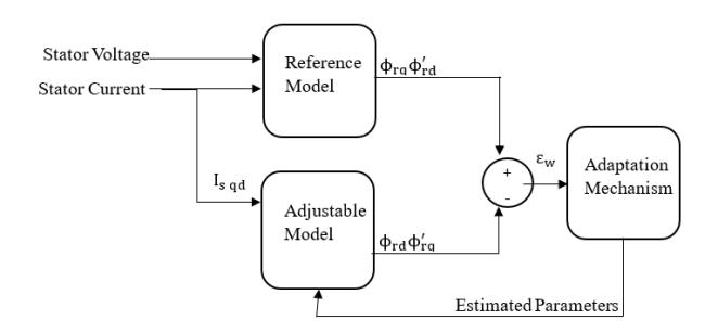
Figure 3 MRAS speed scheme estimator (Fnaiech, Guzinski, Trabelsi, Abdellah, & Benbouzid, 17 April 2021).
The output variable of each model, in this case, the rotor flux, served as the goal state variable for estimation. This entails using the stator equations, which comprise the reference model, to derive rotor flux equation. Concurrently, the electrical speed will be connected to the relevant variable obtained from the rotor equations, forming the model that may be adjusted.
The Reference mechanism
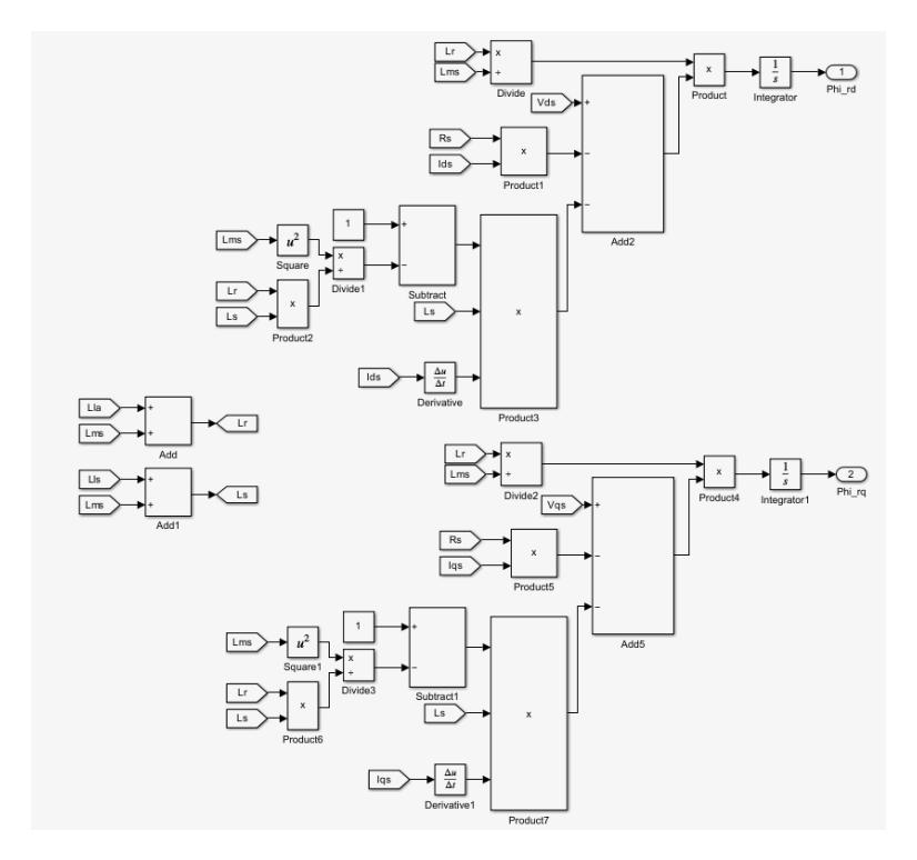
In Figure 10, the MRAS inputs are the stator voltage and current, which are used in the Reference model defined by Eqs. (16) and (17).
\[\frac{\mathrm{d}\phi_{\mathrm{rd}}}{\mathrm{dt}} = \frac{L_{\mathrm{r}}}{L_{\mathrm{ms}}} (V_{\mathrm{sd}} - R_{\mathrm{s}} i_{\mathrm{sd}} - \sigma L_{\mathrm{s}} \frac{\partial i_{\mathrm{sd}}}{\partial t}) \tag{16}\]
\[\frac{\mathrm{d}\phi_{\mathrm{rq}}}{\mathrm{d}t} = \frac{L_{\mathrm{r}}}{L_{\mathrm{ms}}} \left( V_{\mathrm{sq}} - R_{\mathrm{s}} i_{\mathrm{sq}} - \sigma L_{\mathrm{s}} \frac{\partial i_{\mathrm{sq}}}{\partial t} \right) \tag{17}\]
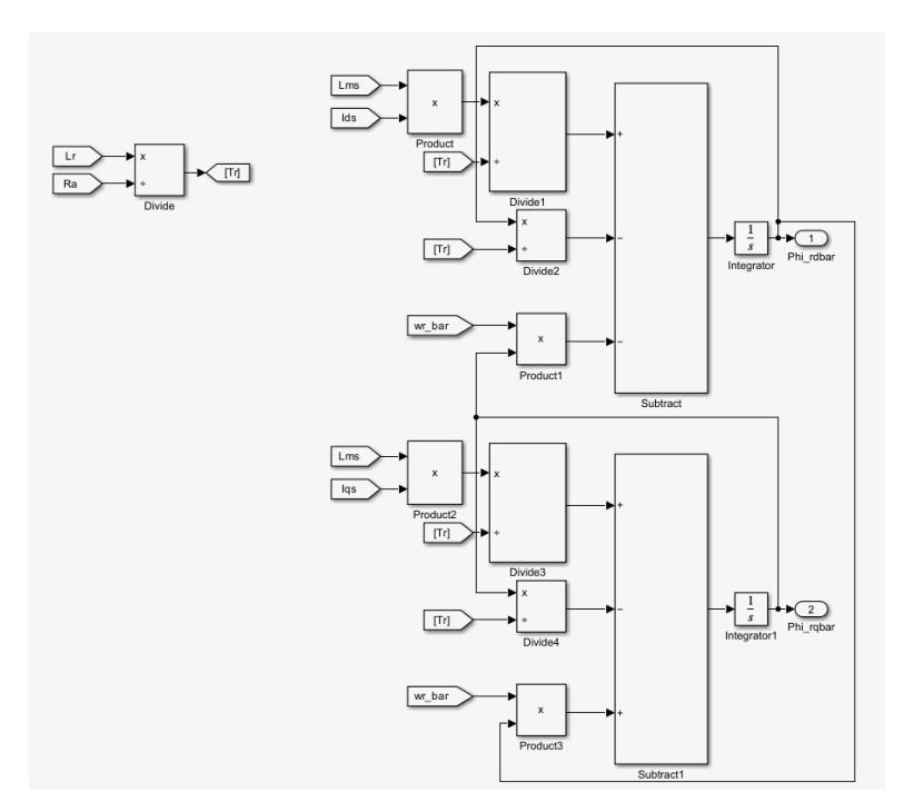
Stator current was also used as input to the adjustable model, which is defined by Eqs. (18) and (19).
\[\frac{\mathrm{d}\phi_{\mathrm{rd}}'}{\mathrm{d}t} = \frac{L_{\mathrm{ms}}}{T_{\mathrm{n}}} i_{\mathrm{sd}} - \frac{\phi_{\mathrm{rd}}'}{T_{\mathrm{n}}} - \omega_{\mathrm{r}}' \phi_{\mathrm{rq}}' \tag{18}\]
\[\frac{\mathrm{d}\phi_{rq}'}{\mathrm{d}t} = \frac{L_{ms}}{T_{r}} i_{sq} - \frac{\phi_{rq}'}{T_{r}} + \omega_{r}' \phi_{rd}' \tag{19}\]
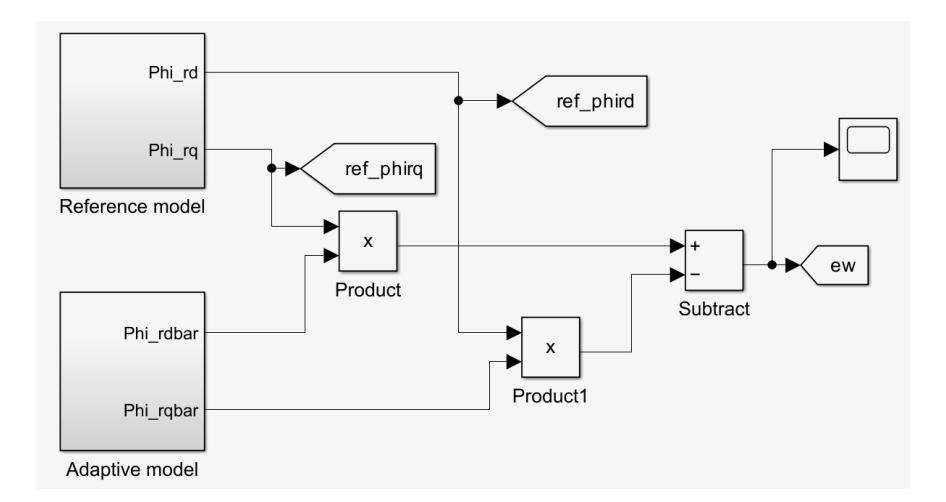
The outputs of the Reference model and the Adjustable model were then combined as per equation 20.
\[\varepsilon_{\rm w} = \phi_{\rm rd} \phi_{\rm rd}' - \phi_{\rm rd} \phi_{\rm rd}' \tag{20}\]
The output variables of the reference and adjustable models are the rotor fluxes. The input of the Adaptation mechanism is the \(\epsilon_w\).
In Figure 3, the error, ε, for the corrector was computed using the cross product, as illustrated in equation 20. The adaptation mechanism involved the FLC and PID.
Fuzzy-PID Regulator
The fuzzy PID regulator combines both PID and fuzzy logic controllers, enabling adaptation to diverse scenarios, including variations in input quantities. The fuzzy PID controller's principal goals were to streamline control methodologies and enhance the system's dynamic and static performance, particularly for systems with complex parameter sets. The fuzzy controller was designed to adjust the PID parameters (Kp, Ki, and Kd) to achieve desired performance metrics, including overshoot, rise time, settling time, and steady-state error. Meanwhile, the PID controller's proportional, integral, and derivative actions were employed to generate the control signal for the fuzzy logic controller. Each controller was designed in MATLAB and combined to form a Fuzzy-PID regulator, illustrated in Figure 4, integrated with MRAS speed estimator.
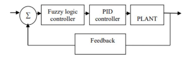
Regulator for fuzzy PID Block diagram.
From Figure 5, the proposed model was observed to begin with the definition of the motor's parameters. The parameters were utilized in the simulation of a single-phase induction motor. The load torque was varied from no load to full load; its rotor speed and electromagnetic torque were observed and plotted. This enabled the development of a sensorless mathematical model for a single-phase induction motor. The stator voltage and stator current of the SPIM were used as input to the MRAS. The difference between the reference and adjustable models formed the error signal. This enabled the estimation of speed for a sensorless single-phase induction motor. The error signal was used in the fuzzy logic controller to make a continuous decision. The chosen control signal from the fuzzy logic was utilized as input in the PID. The PID then calculated the appropriate control signal from the three defined gains (Kp, Ki and Kd). The PID output was a control signal that displayed the estimated speed.
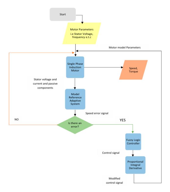
Model flow chart.
Simulation Results
Simulation of Single-Phase Induction Motor
The controller was implemented in MATLAB/Simulink. Tests covered reference steps and load perturbations to assess rise time, overshoot, steady-state error, and IAE. The parameters presented in Table 1 were carefully selected to represent a typical low-power single-phase induction motor (SPIM) widely used in domestic, agricultural, and small industrial applications. The motor rating of 0.5 HP, 220 V, 50 Hz provides a realistic platform for analyzing adaptive speed control performance under variable operating conditions, and these parameters were derived from standard manufacturer data and validated in previous modelling studies. Simulation began with the definition of initial parameters as observed in Table 1.
| Parameter | Value |
|---|---|
| Frequency | 50Hz |
| R_S | 2.02Ω |
| R_a | 7.14Ω |
| R_r^' | 4.12Ω |
| L_ls | 7.4〖*10〗^(-3) H |
| L_la | 8.5*10^(-3) H |
| L_ms | 0.1772H |
| L_lr^' | 5.6*10^(-3) H |
| Input Voltage | 230V |
| K | 1.18 |
| Stator:rotor turns ratio | 1 |
| J | 0.0146kg.m^2 |
| T_L | Vary |
| B_m | 0.0001N.m.s |
| P | 2 pole pairs |
| Disconnection speed | 98% synchronous speed |
Table 1 SPIM parameters
The input voltage was converted to d-q axis form usingEq. (14). This was observed in Figure 6.
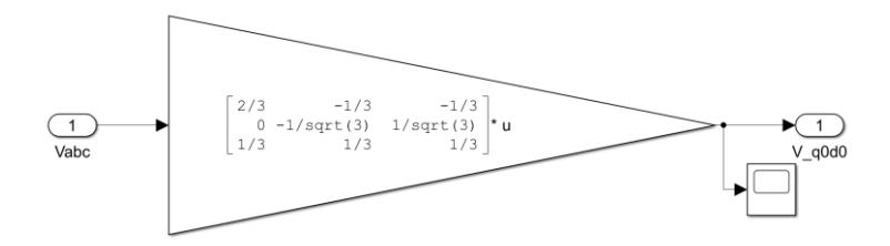
Phase to d-q axis calculation as per Eq. (14).
The fluxes of the stator and rotor were calculated using Eqs. (1) to (4), with Eq. (15) applied in ωr calculation, as shown in Figures 7 and 8, respectively.
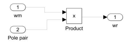
Conversion of Rotor mechanical to Rotor electrical angular velocity as per Eq. (15).
d-q flux calculations as per Eqs. (1) to (4).
The stator and rotor d-q currents were calculated utilizing Eqs. (5) to (8). This was evident in Figure 9.
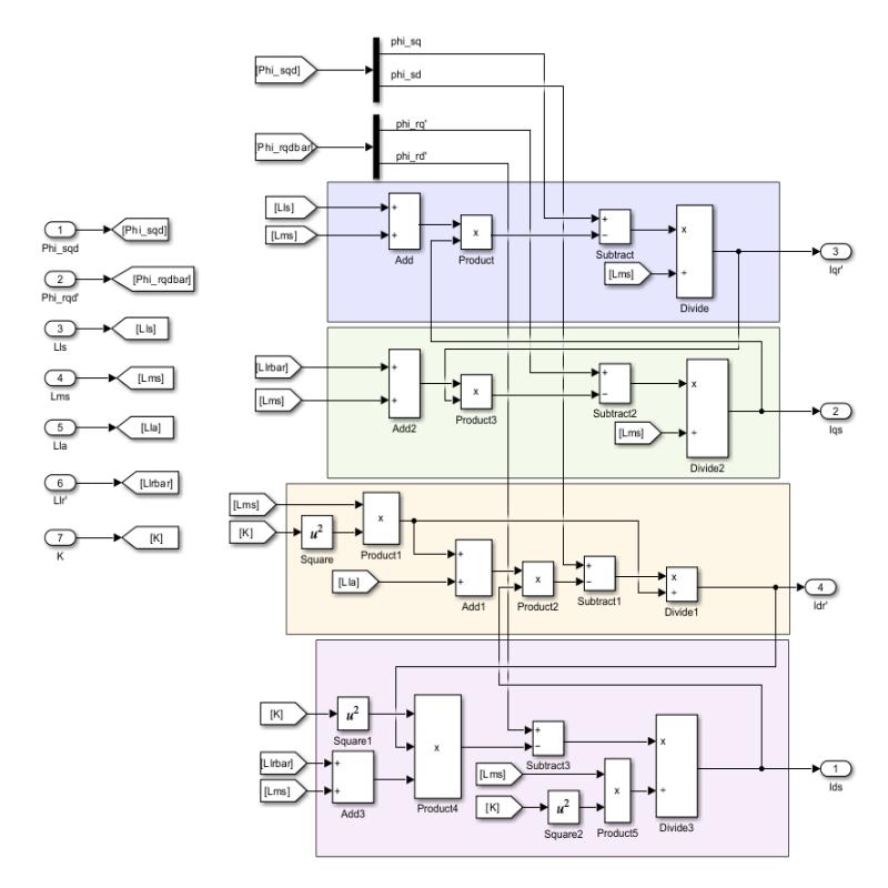
d-q current calculations as per Eqs. (5) to (8).
The rotor speed and electromagnetic torque were then calculated via Eqs. (9) and (10). This is evident in Figure 10.
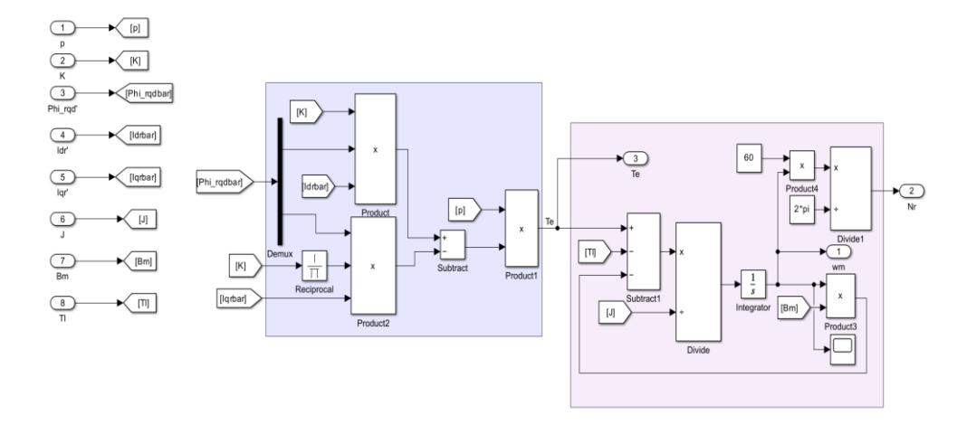
Speed and Torque calculations as per Eqs. (9) and (10).
Finally, the slip was calculated utilizing Eqs. (11) and (12). This is evident in Figure 11.
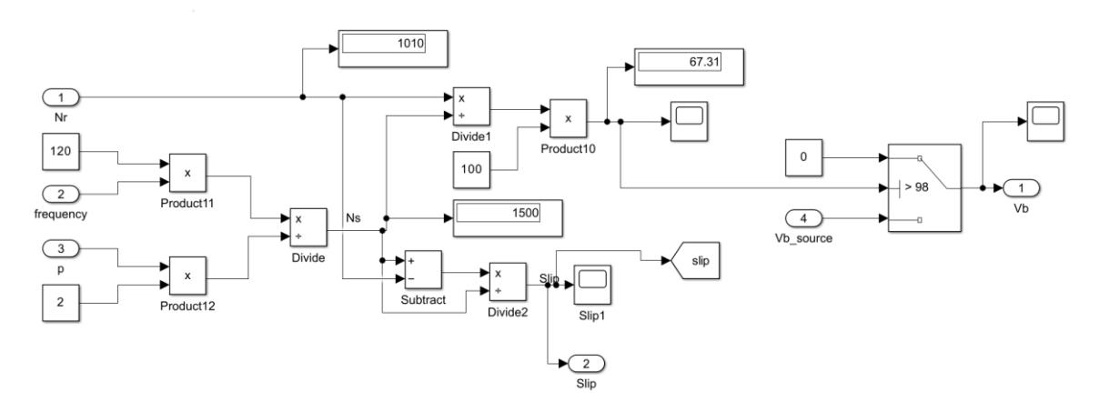
Slip calculation as per Eqs. (11) and (12), and disconnection speed calculation.
The model developed for a sensorless SPIM based on Eqs. (1)-(15) is as follows (Figure 12).
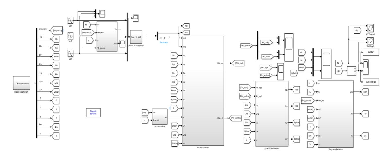
Model developed for a sensorless SPIM based on the Eqs. (1)-(15).
The load torque was then varied from no load to full load, and the graph was observed.
Simulation of the MRAS Model
The stator voltage and the stator current of the SPIM were taken as input to the MRAS, through Eqs. (16) and (17), a model of the reference was made. This is evident in Figure 13.
Reference model calculation simulation as per Eqs. (16) and (17).
Equations 18 and 19 were applied to simulate the adjustable adaptive model. This is evident in Figure 14.
Adaptive System calculation as per Eqs. (18) and (19).
These reference and adaptive models were then combined using equation 20 to form the error signal. This is evident in Figure 15, which contributed to the fuzzy logic controller model.
Model Reference Adaptive System Block diagram simulation and calculation of Eq. (2).
The aim was to establish an integrated MRAS and fuzzy PID control model for speed control of a single-phase induction motor. This model guarantees precise and resilient motor speed control across different speeds as load changes. The research has successfully resulted in accurate speed control of a SPIM follower.
Simulation of FUZZY-PID Model
The Fuzzy-PID regulator was designed to enhance adaptability in the MRAS speed control scheme. The controller uses two input variables: the speed error and its change, both normalized to the range [−1, 1]. Each input variable is represented by three triangular membership functions: Negative (N), Zero (Z), and Positive (P). The output variable is the incremental adjustment applied to the PID gains (Δ, Δ , Δ), which are combined to determine the influence of each term on the control signal.
Simulation of Fuzzy Logic Controller
The controller inputs (the error and the change in error), the output (the control signal), and the state variables (negative, zero, positive) of the plane under consideration were considered. While the complete universe of discourse spanned by each variable was split into a number of fuzzy subsets, each was assigned a linguistic label, as seen in Figure 16.
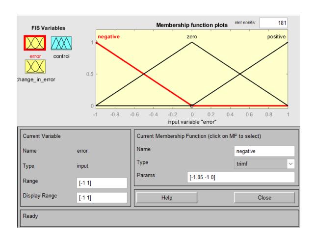
Fuzzy Logic Controller: FIS variables.
Membership function for each fuzzy subset was obtained, then fuzzy relationships were assigned between the inputs or states of fuzzy subsets on one side and the output of fuzzy subsets on the other side, thereby forming a rule base. The fuzzification process was carried out, and the output contributed from each rule using fuzzy approximate reasoning was identified. The fuzzy outputs from each rule were combined, and defuzzification was applied to obtain a crisp output, which enabled the modelling of the PID controller.
Simulation of PID Controller
The blocks for forming equation 20 were placed in MATLAB and connected appropriately, as shown in Figure 17.
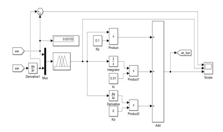
Fuzzy Logic controller integrated with a PID controller diagram
The values of Kp, Ki and Kd were then adjusted to minimize speed error.
Simulation Results Discussion
Single Phase Induction Motor (SPIM)
After modelling the SPIM using Eqs. (1) to (15), the results were observed in Figure 18, the input voltage is specified from the motor specifications. Va1 is the main winding voltage, and Vb1 is the auxiliary winding voltage. The input voltage () was 230V, and that was met on both the main and auxiliary winding. The auxiliary winding was lagging by 90 degrees. This validates the correct representation of SPIM's starting condition.
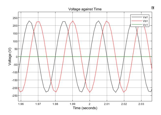
Input Voltage ().
A comparison was presented between the estimated rotor d–q fluxes (′ ) with reference rotor d–q fluxes () generated from the MRAS observer. The results in Figure 19 indicated that the reference rotor fluxes closely track the actual rotor fluxes, showing a high degree of correlation in both magnitude and phase alignment. This demonstrated that the MRAS-based reference model is accurately estimating the components of the rotor flux in the rotating d–q reference frame
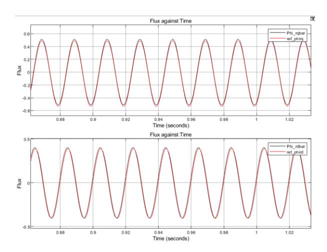
Reference rotor d-q fluxes and Rotor d-q fluxes comparison graphs.
From Figure 20, a comparison between the rotor d-q fluxes and the reference rotor d-q fluxes signals shows that the reference rotor d-q fluxes from the MRAS were almost identical to the rotor d-q fluxes. The comparison confirms that the MRAS reference flux closely matches the actual rotor flux, ensuring the accuracy of the flux estimation required for sensorless control.
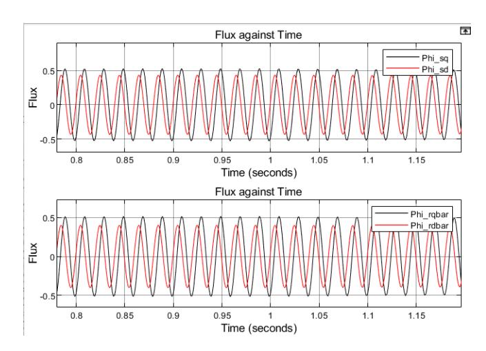
Stator d-q fluxes and Rotor d-q fluxes graphs
From Figure 16, the graphs of the stator d-q fluxes and the rotor d-q fluxes are shown. These are the expected observations of the rotor and stator fluxes in an SPIM, thereby verifying that the motor model is consistent with theoretical flux dynamics.
From Figure 21, the stator d-q currents and rotor d-q currents are shown. These were the expected results for the rotor and stator currents, confirming the accuracy of the SPIM electrical model.
From Figure 22, the speed and torque curves of a SPIM: no load from 0-1 seconds, 1Nm torque from 1-2 seconds, and finally full load (6Nm) from 2-10 seconds. The speed decreased with increasing loading, while the electromagnetic torque increased. The high overshoot at 500 rpm shown here corresponds to the baseline. When the proposed MRAS– Fuzzy-PID is applied under the same reference, overshoot is substantially reduced, consistent with the controller's damping action.
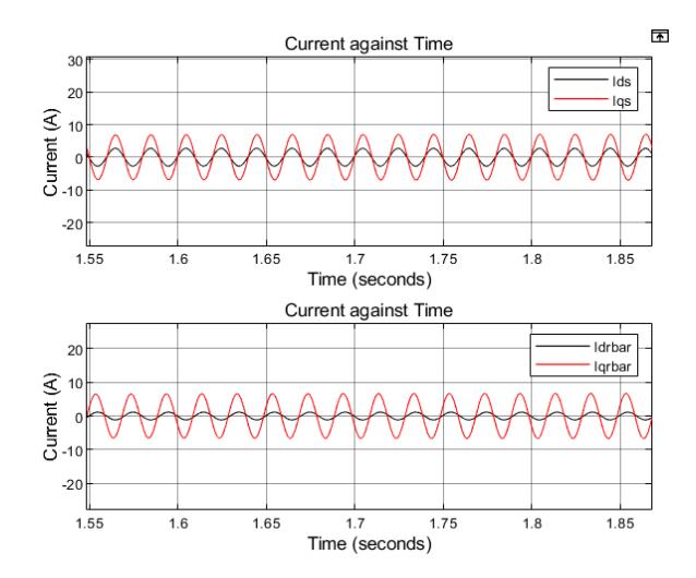
Stator d-q currents and rotor d-q currents graphs.
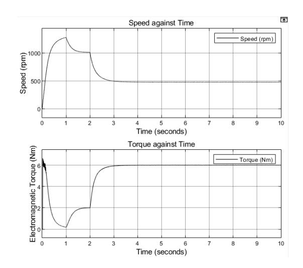
Speed and Torque graphs.
From Figure 23, the slip reduced between 0-1 under no load conditions, when the load was changed into 1Nm, and it slightly increased to a slip of about 33% and when at full load, it finally reached a theoretical slip of 68%, validating theoretical SPIM load–slip characteristics.
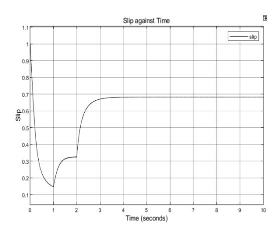
Slip graph.
From Figure 24, the torque increased to the maximum torque or pullout torque of about 6-6.5 Nm as the speed increased. Then the motor's electromagnetic torque decreases because it was initially operating under no-load conditions. After loading, the electromagnetic torque increases as the speed reduces.
From Figure 25, the torque increased to the maximum torque or pullout torque of about 6-6.5 Nm as the slip was reduced. Then the motor's electromagnetic torque decreases because it was initially operating under no-load conditions. After loading, the electromagnetic torque increases with increasing slip.
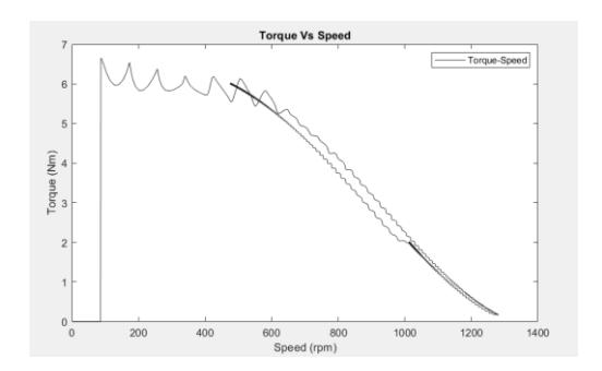
Electromagnetic Torque vs Speed graph.
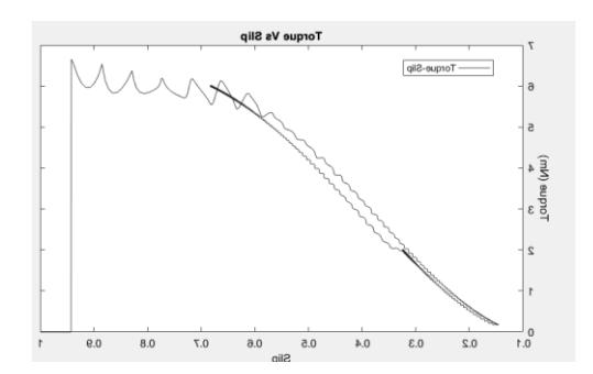
Electromagnetic Torque vs Slip graph.
Model Reference Adaptive System (MRAS)
From Figure 26, the MRAS error output is observed to increase when the load changed from 1Nm to the full load of 6Nm. This shows how off the SPIM was from the reference as the loading increases. There was a high error at the motor's initial start. The least error was observed at no load speeds.
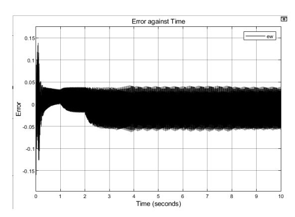
Model Reference Adaptive System graph.
Fuzzy Logic Controller Simulation
The FLC inputs were error with a range of -1 to 1 and a change in error of the speed within -100 to 100, while the output was the controlled output, the rules which were subjected to fuzzy logic controller inputs, which were based on Mamdani inference, as observed in Figure 27 which indicated the validity of the fuzzy rules, as there was no correction from the controller. The controller's output was then fed to the PID.
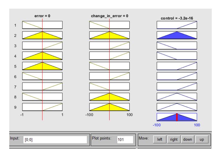
Graphical interface of FLC.
PID Controller Simulation
The PID controller was tuned using a trial-and-error method to set initial values. The response was then optimized by integrating fuzzy logic adjustments. The results show that the Rise time was reduced significantly with increased Kp, the overshoot was minimized with proper tuning of Kd and steady-state error approached zero with increased Ki. Figure 28 illustrates the response of the simulated speed of SPIM controlled solely by a PID controller.
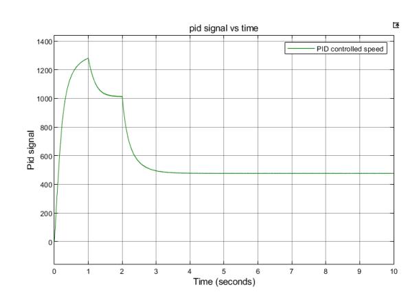
Simulated speed response of SPIM using the PID controller only.
Integrated Simulation
The baseline PID reaches the setpoint but exhibits a longer rise time and notable overshoot; steady-state error persists under a load perturbation, confirming the need for adaptive intelligence.
From Figure 29, the MRAS (ew + change in error) yielded the largest results, the fuzzy logic controller's control output was reduced, and the PID controller's control output was the smallest. Through continuous processing of linguistic logical variables, the error was significantly reduced in the fuzzy logic. Then, through PID gain controls, further reduction in this error was observed. This clearly shows the importance of the MRAS fuzzy-PID controller, as the error has been significantly reduced over the simulation period. Finally, the SPIM was returned to the expected running speeds, with minimal speed fluctuations. Adding fuzzy control improves adaptability and reduces fluctuations versus PID, though overshoot and steady-state error remain non-negligible. The cascade delivers the fastest rise, lowest overshoot, and smallest steady-state error across operating points. Under load steps, speed dip is minimal and recovery is rapid, indicating robust regulation.
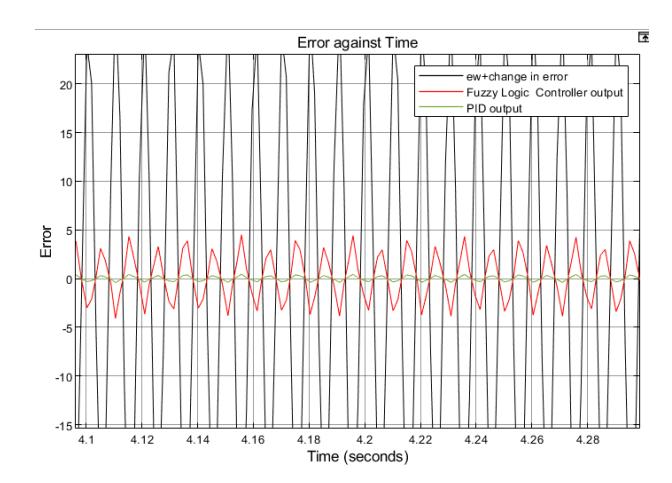
MRAS output (ew + change in error), MRAS+FLC output (Fuzzy Logic Controller output), and MRAS+FLC+PID controller (PID results) results over maximum loading only.
From Figure 30, the MRAS results were the largest, then the fuzzy logic controller's control output was reduced, and finally, the PID controller's control output was the smallest. The controller's adaptability is evident, as it adjusted the error at varying loads, resulting in minimized error. This further confirms the controllers' functionality under both singleand varying-load conditions.
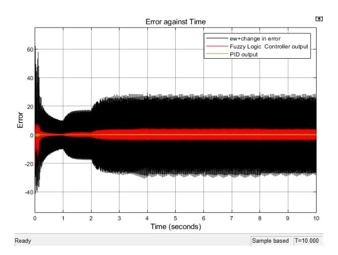
MRAS output (ew + change in error), MRAS+FLC output (Fuzzy Logic Controller output), and MRAS+FLC+PID controller (PID results) results over varying load.
Speed Analysis of the SPIM
To evaluate the efficiency of the proposed MRAS + Fuzzy-PID controller, performance was compared with two benchmarks: the reference system and MRAS integrated with only a Fuzzy Logic Controller (FLC). Table 2 summarizes key performance metrics from the simulations.
Table 2 SPIM Speed Analysis
| Controller | Rise Time (s) | Overshoot (%) | Steady-State Error (%) | IAE |
|---|---|---|---|---|
| PID | 0.48 | 22.4 | 6.12 | 12.5 |
| MRAS + FLC | 0.32 | 15.8 | 3.45 | 8.6 |
| MRAS + Fuzzy-PID | 0.17 | 9.2 | 1.73 | 3.9 |
With PID, MRAS+Fuzzy-PID yields the lowest IAE, confirming the smallest cumulative tracking error over time. Rise time and overshoot are simultaneously reduced, while steady-state error approaches zero, demonstrating both fast and precise regulation. Compared to conventional PID and MRAS+FLC, the proposed MRAS–Fuzzy-PID regulator achieved the lowest IAE, indicating the smallest cumulative tracking error over time. Rise time decreased by 65.5%, overshoot by 58.9%, and steady-state error by 71.8% relative to PID, while overshoot and error were further reduced compared to
MRAS+FLC. This demonstrates that the cascade approach provides both faster and more precise regulation with improved robustness.
Conclusion
In this paper, MRAS Fuzzy-PID controller has been designed to control the speed of a single-phase induction motor. The sensorless SPIM speed-control strategy that cascades MRAS estimation with a Fuzzy-PID regulator. Simulations showed marked performance gains over PID and MRAS+FLC: rise time decreased by 65.5%, overshoot by 58.9%, and steadystate error by 71.8%, with the lowest IAE across scenarios. The cascade structure combines adaptability and precision, ensuring fast, accurate, and robust speed regulation without the need for physical sensors. Future work will focus on experimental validation and embedded implementation.
Acknowledgement
The author is thankful to the Department of Electrical and Electronics Engineering at Murang'a University of Technology for its support.
Nomenclature
| J | Rotor Inertia |
|---|---|
| ωm | Rotor Mechanical Angular Velocity |
| Bm | Friction Coefficient |
| TL | Load Torque |
| Ns | Synchronous Speed |
| Nr | Rotational speed |
| f | Frequency |
| P | Poles |
| Na | Number of Auxiliary Stator Winding |
| Nm | Number of Main Stator Winding |
| ωm | Rotor Mechanical Angular Velocity |
| ωr | Rotor Electrical Angular Velocity |
Compliance with ethics guidelines
The authors declare they have no conflict of interest or financial conflicts to disclose.
This article contains no studies with human or animal subjects performed by the authors.