
Introduction
Pillars are key structural components in coal mining. This is because pillars provide temporary or permanent support for tunnelling and mining operations [1]. Properly designed and stable pillars help prevent mine collapse and associated fatal accidents, while unstable pillars can lead to a range of significant and potentially devastating consequences, including risk to miner safety, financial losses, to mine collapse [2]. Hence, it is important to maintain the stability of underground pillars.
The safety factor (also known as the factor of safety or stability factor) in pillar design is a measure of the structural capacity of a system beyond the expected loads or anticipated conditions. It is calculated as the ratio of pillar strength to pillar stress. According to Li [1] and Lunder [3], rock or coal pillars are regarded as unstable if their safety factor is less than 1 and stable if it is greater than 1. For instance, a safety factor greater than 1 indicates that the pillar's load-bearing capacity is higher than the actual load, suggesting a safety margin that guards against unexpected stress. However, these values are often unreliable, because field uncertainties can sometimes cause changes or inconsistencies in the strength and stress of pillars, potentially compromising their stability and integrity [4]. Hence, unstable pillars often have a safety factor greater than 1 [1].
In general, pillar stability can be divided into two categories: stable/intact and unstable/failed. However, to enhance the insight gained from pillar stability prediction, in this study we also considered the safety factor value to label pillar stability. We used a new safety factor limit and created four labels of pillar stability regarding
the new safety factor limit as in [5]: 1) failed pillars with an SF less than the new limit SF (F0); 2) failed pillars with an SF greater than the new limit (F1); 3) intact pillars with an SF less than the new limit (I1); and 4) intact pillars with an SF greater than the new limit (I0).
Because accurately classifying the areas of pillar stability is crucial in creating safe coal mines, over time researchers have used various methods to assess pillar stability or to find the most suitable pillar design model to maintain pillar stability. Some of these methods are: empirical methods, numerical modeling, and probabilistic modeling. In 2019, Mark and Agioutantis [6] conducted an analysis of coal pillar stability (ACPS) by integrating the three previous pillar stability analysis software packages (ARMPS, AMSS, and CMRR), which are empirical pillar design methods used in almost every coal mine in the US. In 2020, Eremin et al. [7] used the finite-difference method along with continuum damage mechanics (CDM) to estimate the steps of the roof caving in long-wall mines, which is an essential stage in mine design. In 2021, Kumar et al. [4] analyzed the stability of coal pillars using a probabilistic approach, considering cases of stable and failed pillars in India.
In recent years, it has been shown that machine learning techniques have the potential to revolutionize conventional ways of assessing coal pillar stability. This is because machine learning techniques can learn from vast and complex patterns and provide much greater predictive power compared to traditional statistical models [8]. Several machine learning techniques have been used to assess pillar stability. Hidayat et al. [9] used adaptive neuro-fuzzy inference systems (ANFIS) to predict pillar stability and optimal input variables to maximize accuracy. Liang et al. [10] used the GBDT, XGBoost, and LightGBM algorithms to predict pillar stability, achieving an accuracy of 83.1%, 83.1% and 81.69%, respectively. The results also showed that the average pillar stress and pillar width-to-height ratio were the most important factors in the prediction results. Ahmad et al. [11] used random tree, C4.5 decision tree, support vector machines (SVM) and fishery discriminant analysis (FDA) algorithms for pillar stability classification. In 2022, Li et al. [1] showed that the logistic model trees (LMT) algorithm had the highest accuracy among logistic regression machine learning methods (SVM, ANN, Naïve Bayes, Random Forest, J48) on rock and coal pillar data sets.
This study used ensemble learning artificial neural network-backpropagation (ANN-BP) with three activation functions: ReLU, ELU, and GeLU as in Mendrofa et al. [5], as well as a multiclass SVM method with a polynomial kernel and a radial basis function (RBF) kernel. First, the ANN-BP ensemble learning model was used to classify the coal pillars into four categories based on new safety factor limits. Then the multiclass SVM with polynomial kernel and RBF kernel activation functions were implemented to classify the stability area of the new coal pillar categories obtained from the ensemble learning ANN-BP. The proposed model is aimed at providing a simple, quick, and accurate prediction method for classifying coal mine pillar stability and pillar stability areas that is based on calculation and historical observation data.
In this study, the authors used South African coal mining data also used by van der Merwe and Mathey [12] by modifying the two categories of pillar stability (intact and failed) into four categories based on the pillar stability and new safety factor calculations. The remainder of this paper consists of: Section 2. Materials and Methods, Section 3. Implementation, Section 4. Simulation and Analysis, Section 5. Conclusions, Section 6. Acknowledgment and Section 7. References.
Materials and Methods
Materials
South African coal mining data from van der Merwe and Mathey in 2013 [12] were used. It contains four variables: depth to floor, bord width, pillar width, pillar height, and two categories of pillar stability (intact and failed). An additional variable (called ratio), based on Liang et al. [10], is calculated by dividing the pillar width by the mining height. The intact category represents a stable pillar, while the failed category represents an unstable pillar that can cause mine collapse. The data showed that 337 of the 423 pillars were intact. The description of each variable and the data sample is shown in Tables 1 and 2, respectively.
Table 1 South African coal mining data variables description.
| Variable Name | Data Type | Description | Unit Measure |
|---|---|---|---|
| Depth to floor (𝐻) Numeric | Depth of mining below ground level | Meter | |
| Bord width (𝐶) | Numeric | Distance between pillars | Meter |
| Pillar width (𝑤) | Numeric | Width of the pillar | Meter |
| Pillar height (ℎ) | Numeric Height of the pillars from the bottom of the excavation | Meter | |
| Ratio | Numeric | Pillar width to pillar height ratio | - |
Table 2 South African coal mining data sample.
| 𝑯 | 𝑪 | 𝒘 | 𝒉 | Ratio Stability | |
|---|---|---|---|---|---|
| 76.2 | 6.1 | 4.88 | 1.37 | 3.56 | Failed |
| 29 | 6.3 | 5.4 | 2.9 | 1.86 | Failed |
| 60 | 6 | 7 | 1.82 | 3.85 | Failed |
| 55 | 5 | 7 | 2.2 | 3.18 | Failed |
| 98.15 | 5.23 | 12.56 | 2.65 | 4.74 | Intact |
| 64.79 | 5.37 | 13.03 | 3.08 | 4.23 | Intact |
| 61.1 | 6.61 | 7.08 | 4.49 | 1.58 | Intact |
| 42 | 6.78 | 5.38 | 3.96 | 1.36 | Intact |
Methods
In designing pillars and measuring their stability, the safety factor (SF) is often used as an aid for quantitative analysis. SF is often defined as the ratio of pillar strength to pillar stress. An appropriate method for calculating the strength and stress is required for a safe and effective design [13], with SF defined as in Eq. (1):
\[SF = \frac{S_p}{\sigma_p},\tag{1}\] where is the pillar strength and is the pillar stress. There are some calculations for pillar strength [14], and this study used a value for that fulfills Eq. (2) 12]:
\[S_p = 5.47 \, w^{0.8} / h \, MPa, \tag{2}\] where w is the pillar width (m), h is the pillar height (m), and 5.47 is the strength of the coal (MPa). Pillar stress () is defined as in Eq. (3) [15]:
\[\sigma_p = \frac{25HC^2}{w^2} kPa, \tag{3}\] where is the depth to the base of the mine (m), is the sum of the pillar width and the distance between pillars (bord width) in meters, and 25 is the product of the density and gravity (kPa/m).
According to Li et al. [1] and Lunder [3], the commonly used SF limits are often unreliable because many unstable pillars have an SF greater than 1. This study also modified the two pillar stability categories (intact and failed) into four categories [5]: 1) failed pillars with an SF less than the limit (F0); 2) failed pillars with an SF greater than the limit (F1); 3) intact pillars with an SF less than the limit (I0); and 4) intact pillars with an SF greater than the limit (I1). The new SF limits used to modify the data categories were defined as in Eq. (4):
\[Limit = \frac{Avg.SF\ Failed + Avg.SF\ Intact}{2} = 2.23,\tag{4}\] where Avg.SF Failed and Avg.SF Intact were obtained by calculating the average of all pillar SF values in the failed and intact categories.
The ensembled ANN-BP is an implementation of ensemble learning methods on the ANN-BP model. The ANN models are part of a deep neural network comprising multiple hidden layers (MLP) [16,17]. The basic ensemble algorithm selected is bagging, which is commonly referred to as bootstrap aggregation. Bagging involves creating an independent observation sample using the same training dataset. This sample is used to train every basic model used in ensemble learning. Samples can be made with or without replacement [18]; this study used replacement when creating samples. The ensemble output used was based on the output of each basic model used based on majority vote.
The three basic models used were ANN-BP with three different activation functions: ReLU, ELU and GeLU on the hidden layers. The reason for choosing these three activation functions was: ReLU is more effective because only some of the neurons are stimulated at once, instead of all of them [19]. However, according to Rasamoelina et al. [20], the drawback is that ReLU may suffer from the problem of dying. Meanwhile, ELU, can reduce the effects of vanishing gradients. Finally, GeLU is a state-of-the-art activation function proposed by Hendrycks and Gimpel [21]. Based on the empirical evaluation of GeLU, ReLU and ELU, GeLU yields superior performance compared with ReLU and ELU. The mathematical formulas for ReLU, ELU, and GeLU are further explained in [20-22].
In the ANN output layer, the softmax activation function, which consist of several sigmoid functions, is used to determine the possibility of input X being in a specific category. The output of the softmax function \(\sigma(X)_j\) for class j given an input \(X = \{x_1, x_2, ..., x_K\}\) is defined as in Eq. (5)[19]:
\[\sigma(X)_{j} = \frac{e^{X_{j}}}{\sum_{k=1}^{K} e^{X_{k}}} , j = 1, ..., K,\] (5)
where K denotes the number of categories. The value of \(\sigma(X)_j\) represents the probability of input X being in category j.
Artificial Neural Network-Backpropagation (ANN-BP) is a feed-forward neural network that uses backpropagation learning algorithms. Backpropagation algorithms are the most commonly used learning algorithms for training neural networks [23], with these algorithms updating the weight and bias in neural networks by minimizing errors.
The ANN-BP training process comprises two stages: feed-forward and backpropagation. In the feed-forward stage, the ANN-BP in this research classifies input \(X = \{x_1, x_2, x_3, x_4, x_5\}\) into certain categories based on the largest value of softmax \(\sigma(X)_j\) resulting from Eq. (5), where j = 0,1,2,3. In the backpropagation process, the weights and biases are updated. Backpropagation begins by calculating the error in the output generated by the feed-forward process using categorical cross-entropy (CCE) with the following general function in Eq. (6) [24]:
\[CCE = -\log(v_i). \tag{6}\] where \(y_i\) is the probability of input X in the ANN-BP falling into category i, calculated using the softmax function. Next, we calculate the total CCE for every \(y_i\), followed by updating the weight and bias. The stages of feedforward and backpropagation in the ANN-BP training with one hidden layer can be seen in more detail in [25].
The evaluation of the classification results uses a confusion matrix [26] to determine: 1) overall accuracy (OA), which is defined as the proportion of occurrences correctly predicted by the model relative to the total number of occurrences. For example, \(r_{ij}\) (where i and \(j=1,2,\ldots,m\)) is a combination of observation frequencies predicted to be in class i and that are actually in class j. Therefore, OA is calculated as in Eq. (7) [27]:
\[OA = \left(\frac{1}{n}\sum_{i=1}^{m} r_{ii}\right),\tag{7}\] where n is the total number of occurrences; 2) recall is defined as the positive class in the problem divided by the number of actual positives (true positives and false negatives); and 3) precision is defined as the positive class in the problem divided by the number of predicted positives (true positives and false positives). According to Gong [24], recall or precision alone is not sufficient for determining the performance of a model during classification. Therefore, this study also used the F-measure (\(F_{\beta}\)), a performance metric that balances recall and precision. The general equation for \(F_{\beta}\) is [26]:
\[F_{\beta} = (1 + \beta^2) * \frac{Precision*Recall}{\beta^2*Precision+Recall'}\] (8)
where \(\beta\) is the factor that determines how important recall is compared to precision. This study used the value of \(F_1\), the harmonic average of precision and recall, which is defined as in Eq. (9):
\[F_1 = 2 * \frac{Precision*Recall}{Precision+Recall}.\] (9)
In \(F_1\), the precision and recall are equally important. Therefore, \(F_1\) can be interpreted as the ability of the model to accurately identify positive cases from all cases.
Based on the explanation of the F1 category, pillars in this category are most likely to be dangerous because, although their SF is classified as intact, the pillars themselves fail. Thus, in this study, we assume that it is much worse to miss an F1 category prediction than to give a false alarm in the other categories. This viewpoint has the same meaning as the need to minimize the number of false negatives in all pillars in the F1 category. In other words, the recall value in F1 is prioritized over its precision value. Therefore, this study also used F-measure \((F_{\beta})\), where \(\beta=2\) in Eq. (8) in the implementation.
For nonlinearly separable data, there are two stages in SVM. The first is to add a soft margin to the optimization problem to anticipate the presence of outliers. This is followed by the use of the kernel function to transform the data into a space with higher dimensions so that it can be classified more easily [28].
The general form of the SVM model is as in Eq. (10) [28]:
\[y(\mathbf{w}) = \mathbf{w}^T \mathbf{x} + b, \tag{10}\] where w is the weight parameter, x the input vector, and b the bias. The primal optimization model for a non-linear SVM with the addition of soft margins can be made by adding a slack variable, \(\xi_i\). Therefore, the model can be written as:
\[min\frac{1}{2}\|\mathbf{w}\|^2 + C\sum_{i=1}^n \xi_i,\tag{11}\] with the constraints
\[y_i(\mathbf{w}^T x_i + b) \ge 1 - \xi_i, \ \xi_i \ge 0, \forall_i = 1, 2, ..., n,\] (12)
where \({\bf w}\) is the weight vector orthogonal to the hyperplane, \({\bf x}\) is the input vector on training data, b is the bias that is the distance from the origin to the hyperplane, \(\xi_i \geq 0\) is the slack variable, and \(C \geq 0\) is the penalty parameter.
Eq. (12) is the primal optimization problem, which has the following dual optimization problem in Eq. (13):
\[\max_{\alpha} \left( \sum_{i=1}^{n} \alpha_i - \frac{1}{2} \sum_{i=1}^{n} \sum_{i=1}^{n} \alpha_i \alpha_j y_i y_j (\boldsymbol{x}_i, \boldsymbol{x}_j) \right), \tag{13}\] with the following constraints in Eq. (14):
\[\sum_{i=1}^{n} \alpha_i y_i = 0, 0 \le \alpha_i \le C, \forall_i = 1, 2, \dots, n.\] (14)
This research uses two kernel functions as in Eq. (15) [28]:
Polynomial Kernel: \[K(\mathbf{x}_i, \mathbf{x}_j) = (\gamma(\mathbf{x}_i, \mathbf{x}_j) + r)^d\], (15)
where d is the polynomial degree, and \(\gamma\) and r are the parameters.
Radial Basis Function (RBF) Kernel:
\[K(\mathbf{x}_{i}, \mathbf{x}_{j}) = exp\left[-\gamma \|\mathbf{x}_{i} - \mathbf{x}_{j}\|^{2} + C\right], \gamma > 0,\] (16)
where \(\gamma\) and C are the parameters. Using the kernel function, Eq. (13) can be written as follows:
\[\max_{\alpha} \left( \sum_{i=1}^{n} \alpha_i - \frac{1}{2} \sum_{i=1}^{n} \sum_{i=1}^{n} \alpha_i \alpha_j y_i y_j K(\mathbf{x}_i, \mathbf{x}_j) \right), \tag{17}\] with the constraints:
\[\sum_{i=1}^{n} \alpha_i y_i = 0, 0 \le \alpha_i \le C, \forall_i = 1, 2, \dots, n,\] (18)
and Eq. (10) can be written as follows:
\[y(\mathbf{w}) = \sum_{i=1}^{n} \alpha_{i}^{*} y_{i} K(\mathbf{x}_{i} \cdot \mathbf{x}_{i}) + b^{*}, \tag{19}\] where \(\alpha_i^*\), \(b^*\) are solutions that fulfil the Karush-Kuhn-Tucker (KTT) conditions, \(K(x_i, x_j)\) is a kernel function, and n is the number of the support vectors (see [29] for further details).
This research used an SVM classifier with polynomial and radial basis function (RBF) kernel functions. Classifier results can be combined in two ways: one-versus-all (OVA) and one-versus-one (OVO) [30]. This study used the OVA approach, with four categories (because there are four data categories resulting from the implementation of the ANN-BP ensemble), where the i th classifier is trained to separate the samples in the i th class from the other samples. The final prediction of this approach is based on the result where the classifier has the highest value [30]:
Class = \[arg max f_i\], (20)
where is the amount of trust generated by the i th classifier.
Before implementing multiclass SVM, hyperparameter tuning is carried out. This research used Bayesian optimization (BO). BO was chosen because it has become a successful tool for hyperparameter optimization of machine learning algorithms, such as SVM and deep neural networks [31]. Bayesian optimization is an iterative algorithm used for hyperparameter tuning in machine learning models [32]. BO aims to determine the optimal hyperparameters of a model by building a probabilistic model (surrogate function) to model the relationship between the hyperparameters and the performance of the model [33]. It then relies on an acquisition function, such as the upper confidence bound (UCB), to guide the search for optimal hyperparameters [32,34]. The more detailed steps in the BO algorithm are as follows:
- 1. The interval for each hyperparameter to be tuned is determined. In this study, we tuned every hyperparameter used in the kernel functions and SVM objective function. The initial set of hyperparameters, , was selected by choosing five random parameter combinations from each given interval.
- 2. Using each parameter combination , = 1, 2, … , , the SVM model is trained, and the model performance is evaluated using five-fold cross validation as the model performance metric as well as the objective function of the BO algorithm ().
- 3. A surrogate function () is chosen to estimate the model performance for different hyperparameters based on previous evaluations and to update the model [35]. In this study, Gaussian processes were used as surrogate functions. It is assumed that the probabilities ((1 ), (2 ), … , ( )) for the finite parameters 1 , 2 . … , ∈ follow a multivariate normal distribution, represented as follows:
\[p(f) = p(f(x_1), \dots, f(x_n)) \sim N(\mu(x), k(x_i, x_j)),\] (21)
where () is the mean function, and ( , ) is the covariance function [35].
4. A new parameter +1 is selected using the acquisition function. To maximize the objective function, we used the UCB as our acquisition function [32]. The UCB equation is expressed as follows:
\[\alpha(x) = UCB(x) = \mu(x) + \kappa \sigma(x), \tag{22}\] 5. where () is a standard deviation function [34] and ≥ 0. The new parameter +1 is selected using the following equation [35]:
\[x_{n+1} = arg \max_{x} \alpha(x, D_n). \tag{23}\]
6. Repeat step 2 to 4 until the stopping criterion is met or the maximum number of iterations is reached. At the end of the process, the hyperparameters that maximize the performance of the model are selected.
Implementation
In the implementation, we began by modifying the categories of the data as follows: 1) use variable values from each pillar of the data to calculate the SF value of every pillar using Eq. (1); 2) use every SF value from every failed and intact pillar to calculate the new SF limits using Eq. (4); 3) use the new limit of 2.23 to classify pillar stability into four categories: a) F0: Failed & < 2.23; b) F1: Failed & ≥ 2.23; c) I0: Intact & ≥ 2.23; d) I1: Intact & < 2.23. The F0 and I0 pillars were treated as cases of normal pillar stability, in which the pillar stability categories matched their safety factors. Pillars F1 and I1 pillars were treated as cases of anomalous pillar stability. For example, F1 pillars are those that have failed despite having an SF higher than the SF limit.
The results of modifying the categories in the data created an imbalance, with the number of pillars in the F0, F1, I0, and I1 categories being 67, 19, 209, and 128 respectively. Therefore, oversampling was used to overcome the data imbalances. Oversampling was performed on the data before training the ANN-BP model to preserve valuable information in the majority data class, thereby allowing the model to better learn the data characteristics of minority classes. The synthetic minority oversampling technique (SMOTE) [36] was used. After oversampling, the number of cases in each category was equal to the number of cases in the majority class before oversampling (209 cases).
Following oversampling, label encoding was performed for each category. This was necessary because the ANN-BP cannot process categorical data types. Therefore, F0 = 0, F1 = 1, I0 = 2, and I1 = 3. After category modification, oversampling, and label encoding, the data used had the following variables: depth to floor, pillar height, bord width, pillar width, ratio, stability category (failed and intact) and category label (0,1,2,3).
The next step involved data training, validation, and testing. Four combinations of data proportions were used: 1) 80% training, and 20% testing; 2) 70% training, and 30% testing; 3) 80% training, 10% validation, and 10% testing; and 4) 70% training, 15% validation, and 15% testing. The architecture of the ANN-BP is shown in Figure 1.
Five input neurons in the input layer represent the depth to floor, pillar height, bord width, pillar width, and ratio, with the four outputs being labels 0, 1, 2, and 3. There were four hidden layers, and the numbers of neurons in each hidden layer were 512, 256, 256, and 128.
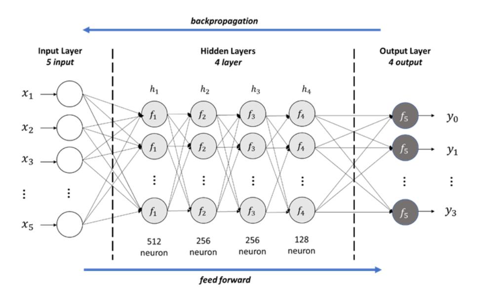
Figure 1 ANN-BP architecture.
The process of ANN-BP ensemble learning begins with sampling with replacement (bootstrapping) of the training data to create new training data from the three basic ensemble learning ANN-BP models. The three bootstrapping percentages were 70%, 80%, and 90%. Bootstrapping was performed for all four proportions of the data. For example, if the proportion of training data is 80% and the bootstrapping percentage is 70%, the initial dataset chosen randomly is 80% of the training data and 20% of the testing data. Bootstrapping was then performed with a total sample of up to 70% of the training data. In the implementation, if the classification results of the three basic models are different, then the majority vote chooses the smallest label, 0 (F0). F0 is the best choice, as F0 is the category with the lowest risk of false predictions compared to the other categories (F1, I0, and I1), because the stability of the F0 pillars in this area is consistent with their expected stability based on their SF.
Simulation and Analysis
The model was simulated using Python. Models with data proportions of 1 and 2 were trained using the early stopping accuracy with a patience value of 10, which stopped the training process after 10 epochs if the training accuracy value did not improve. Models with data proportions of 3 and 4 with validation data were trained using an early stopping validation loss with a patience of 10, which stopped the training process after 10 epochs if the validation loss value did not improve.
The implementation was performed in two stages: 1) using ensemble learning ANN-BP to classify pillar stability into four new categories and; 2) with multiclass SVM using the polynomial kernel and RBF kernel activation functions to determine the classification of areas of pillar stability.
The implementation of the ensemble ANN-BP on the data was performed by modifying the new categories into four categories (F0, F1, I0, and I1) based on the calculations of the limit in Eq. (4). Subsequently, the average and standard deviation of the accuracy of the ensemble learning model were calculated for each proportion of data for each bootstrapping percentage. The average accuracy from 10 experiments in the ensemble learning ANN-BP with the following percentages for each data proportion is shown in Table 3: 1) bootstrapping 70% (EL 70%), 2) bootstrapping 80% (EL 80%), and 3) bootstrapping 90% (EL 90%).
Table 3 Average accuracy of the ensemble learning ANN-BP model.
| Proportion | EL 70% | EL 80% | EL 90% |
|---|---|---|---|
| 1 | 89.88% | 89.29% | 89.29% |
| 2 | 90.20% | 89.44% | 88.73% |
| 3 | 92.98% | 92.14% | 92.86% |
| 4 | 87.94% | 89.37% | 89.29% |
The highest average accuracy from the ensemble learning ANN-BP was obtained with a bootstrapping percentage of 70% and a data proportion of 3, with a value of 92.98%. Therefore, the model could provide an accurate prediction of the pillar stability for approximately 92.98% of the test data used. In other words, the probability of the model making a correct prediction for the test data was 92.98%.
The standard deviation of the accuracy of the ten experiments using ensemble learning ANN-BP is presented in Table 4.
Table 4 Standard deviation of accuracy of the ensemble learning ANN-BP model.
| Proportion | EL 70% | EL 80% | EL 90% |
|---|---|---|---|
| 1 | 1.12% | 0.56% | 1.64% |
| 2 | 0.96% | 0.63% | 1.33% |
| 3 | 1.43% | 1.00% | 1.59% |
| 4 | 1.62% | 1.25% | 1.07% |
The standard deviation of the accuracy of the ensemble learning ANN-BP algorithm was between 0.56% and 1.64%, with the lowest accuracy standard deviation of 0.56% being obtained by EL 80% on the first data proportion, and the highest accuracy standard deviation of 1.64% was obtained by EL 90% on the first data proportion.
In addition to the average accuracy and standard deviation of accuracy, the value of 1 for each category in the data class was calculated. This was performed to determine the overall capability of each model to accurately identify positive cases. Figures 2 to 5 show the results of calculating 1 for each data proportion in each class category.
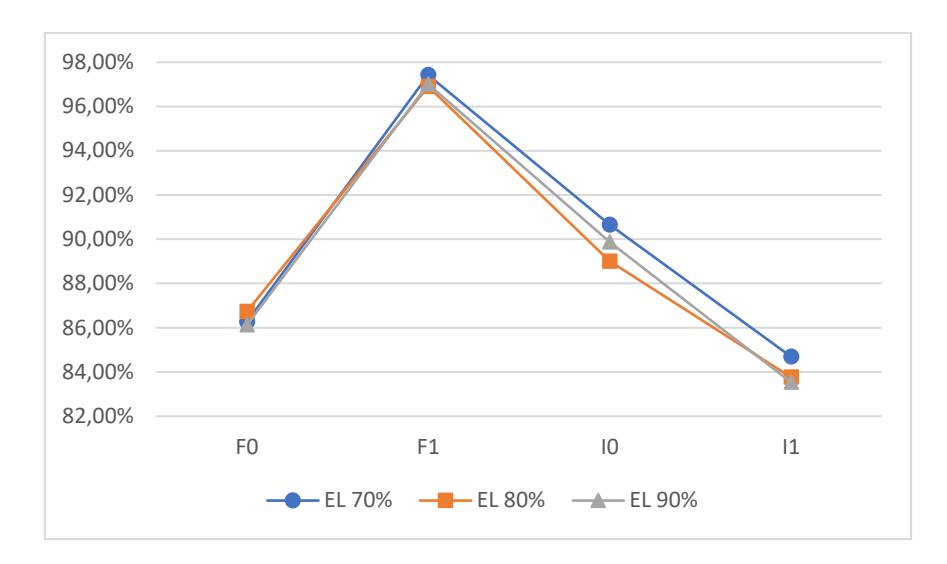
Figure 2 1 values in data proportion 1.
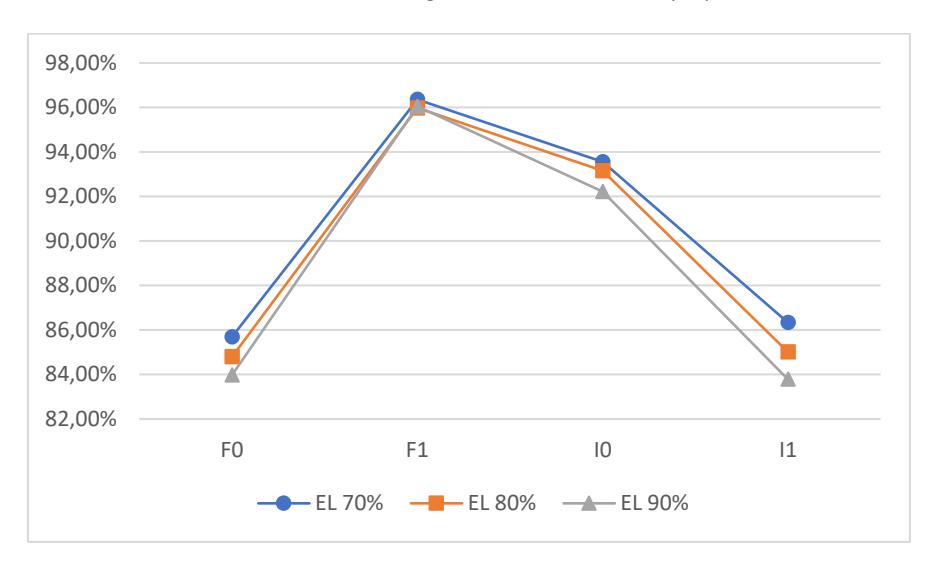
Figure 3 1 values in data proportion 2.
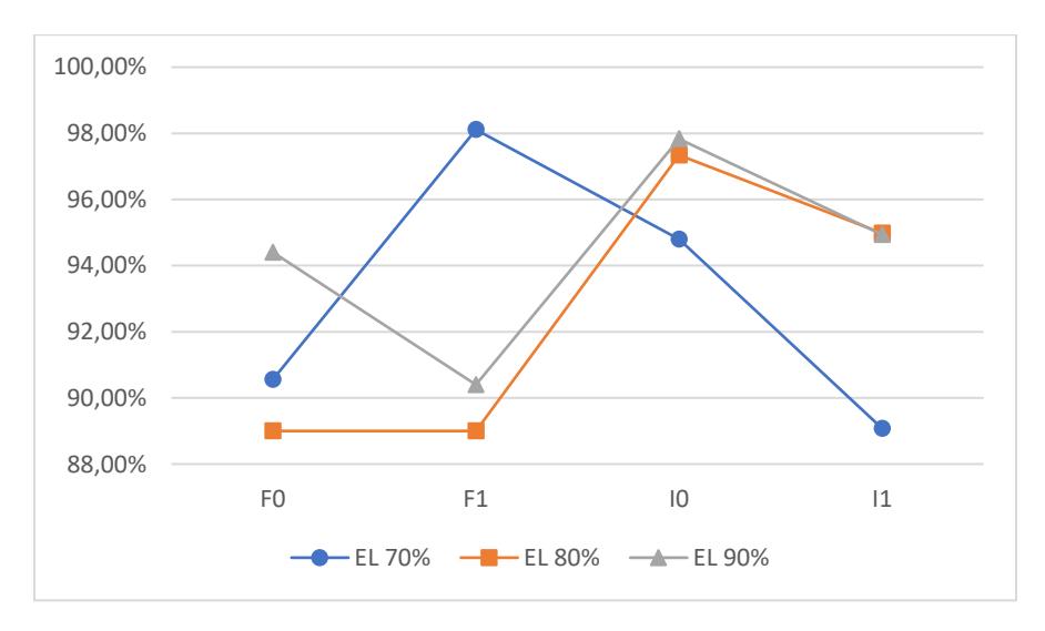
Figure 4 1 values in data proportion 3.

Figure 5 1 values in data proportion 4.
Based on Tables 3 to 4 above, the ensemble learning ANN-BP model provided satisfactory performance (at least 80%) in detecting stability in every category for all data proportions. The best 1 value from the ensemble learning ANN-BP was obtained from data proportion 3 with a bootstrapping percentage of 70%, as follows: the 1 values from classes F0, F1, I0 and I1 were 90.56%, 98.11%, 94.80%, and 89.08% respectively.
Because this study highlighted the importance of the number of false negatives in all pillars in the F1 category, based on the results from Figures 2 to 5 above, the calculation of the number of false negatives from every pillar was only performed in the F1 category. Accordingly, in Table 5, the values of 2 in the F1 category for all the proportion data were as follows:
Table 5 2 values on F1 category
| Proportion | EL 70% | EL 80% | EL 90% |
|---|---|---|---|
| 1 | 98.95% | 98.61% | 98.78% |
| 2 | 98.51% | 98.35% | 98.38% |
| 3 | 98.38% | 96.35% | 97.12% |
| 4 | 97.72% | 98.42% | 98.41% |
From Table 5, the value of 2 in category F1 obtained using the ensemble learning ANN-BP was 98.95% (EL 70%). Therefore, the ensemble learning model shown is very capable in detecting the false negatives in the F1 category.
Based on the results of the overall model evaluation using the average, 1 , and 2 values, the ensemble learning ANN-BP model with a bootstrapping percentage of 70% yielded a better result than the same model with bootstrapping percentages of 80% and 90%, although the difference was not significant (less than 1%). This is because the ensemble learning ANN-BP model with a bootstrapping percentage of 70% is the best at finding variations in data, thereby yielding more robust prediction results for various data proportions and testing data variations.
In short, in the process of determining the classification of new categories on the data used (F0, F1, I0 and I1), the ensemble learning ANN-BP method predicted all four categories very well over 10 attempts, with an average accuracy of 92.98% and an accuracy standard deviation of 0.56 to 1.64%. To observe the overall capabilities of the model in catching positive cases (recall) accurately from all captured cases (precision), the 1 value for each category of data also showed satisfactory performance (at least 80%). The best 1 values from the ensemble
learning ANN-BP were obtained using data proportion 3 with a bootstrapping percentage of 70%, with the F0, F1, I0, and I1 classes yielding values of 90.56%, 98.11%, 94.80%, and 89.08% respectively.
The second part of the implementation involves implementing a multiclass SVM with polynomial kernel and RBF kernel activation functions to determine the stability area of new categories obtained from the ensemble learning ANN-BP method. Based on the new classification categories, imbalanced data (F0, F1, I0, and I1) were obtained; therefore, SMOTE was required. Subsequently, the model parameters were optimized using BO.
The search range in SVM parameter optimization with the polynomial kernel activation function is \(\gamma=(0,2)\), C=(1,2), \(polynomial\ degree=(2,3)\), coefficient=(0,2). The search range in SVM with RBF kernel is \(\gamma=(0,2)\), C=(1,2). The results of SVM parameter optimization with the polynomial kernel activation function were: C=1.574, coefficient=0.59924, polynomial degree=3, \(\gamma=0\). In the implementation, \(\gamma=0.574\) cannot be zero; therefore, the gamma value used is 'auto' or \(\frac{1}{no.\ of\ features}=\frac{1}{2}\). In SVM with RBF kernel, the optimal parameters are \(\gamma=0.5329\), C=2. Theoretically, pillar stability is calculated based on comparisons between pillar strength \((S_p)\) and pillar stress \((\sigma_p)\). Therefore, these two variables are the focus of both the implementation of the multiclass SVM and BO. Tables 6 and 7 show the evaluation of pillar stability area classification results.
Table 6 shows that the accuracy of the multiclass SVM with the polynomial kernel (model Type 1) was 91%, while Table 7 shows that the accuracy of the RBF kernel function was 92% (model Type 2). The precision of each category (F0, F1, I0, and I1) for model Type 1 ranged from 79% to 100%, while for model Type 2, it ranged from 85% to 100%. The recall and \(F_1\)-score for each model are listed in Tables 6 and 7.
In the explanation of category F1, it can be assumed that the pillars in this category had the greatest potential to be dangerous. Tables 6 and 7 also show that the recall values for category F1 were 100%. Thus, each model captured the category F1 in the data very well.
Table 6 Results of evaluation of classification of areas of pillar stability with multiclass SVM polynomial kernel.
| Category | Precision | Recall | F1-score |
|---|---|---|---|
| F0 | 0.95 | 0.97 | 0.96 |
| F1 | 0.79 | 1.00 | 0.88 |
| 10 | 1.00 | 0.67 | 0.80 |
| I1 | 0.98 | 0.96 | 0.97 |
| OA | 0.91 |
Table 7 Results of evaluation of classification of areas of pillar stability with multiclass SVM RBF kernel.
| Category | Precision | Recall | F1-score |
|---|---|---|---|
| F0 | 0.90 | 0.97 | 0.94 |
| F1 | 0.85 | 1.00 | 0.92 |
| 10 | 1.00 | 0.78 | 0.88 |
| I1 | 0.98 | 0.92 | 0.95 |
| OA | 0.92 |
The \(F_1\) value in category F1 for model types 1 and 2, were 88% and 92% respectively. The precision values were 79% and 85% for Models 1 and 2, respectively. Finally, the minimum expected number of false negatives in the F1 category, as determined using F-measure \((F_\beta)\) with a value of \(\beta=2\) in Eq. (4), were 94.9% for model Type 1 and 96.6% for model Type 2. This implies that model Type 2 could capture pillars in category F1 with the potential to be 1.7% more dangerous than model Type 1. Hence, the results of the stability area classification for both models were very good. In this case, Model 2 provided better results than those of Model 1, but not by a significant amount.
To summarize, the process of determining the classification of areas of pillar stability using the multiclass SVM method with a polynomial kernel function had an accuracy of 91%, compared with 92% with an RBF kernel
function. Based on the new pillar category classification, the multiclass SVM method with the RBF kernel function captured 96.6% of the F1 pillars, which have the potential to be dangerous at some point.
To show the classification of stable areas in coal mines, the above results are supported by visualizations. Figure 6 shows a visualization of the pillar stability area classification with a multiclass SVM using a polynomial kernel and RBF kernel.
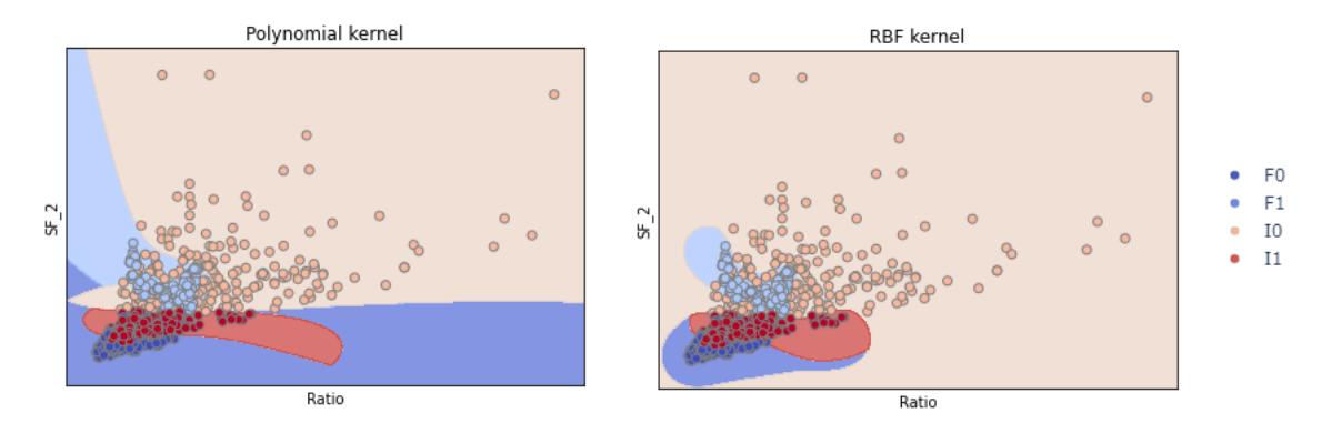
Figure 6 Visualization of pillar stability area with multiclass SVM using polynomial kernel (left) and RBF kernel (right).
Figure 6 shows that in the I1 area, the intact pillars had an SF below the limit, and the failed pillars had an SF below the limit (F0). Furthermore, in the F1 area, the failed pillars had a SF higher than the limit, and the intact pillars had a SF higher than the limit (I0).
The classification areas shown in Figure 6 are consistent with the results shown in Tables 8 and 9 for the classification of areas with pillars in the I1 and F0 categories. However, this SVM model using the RBF kernel function model is more capable of classifying areas within the F1 pillar category than those within the I0 pillar category. In other words, the multiclass SVM model using the RBF kernel function is more capable of classifying failed pillars with a SF higher than the limit compared with an equivalent model using the polynomial kernel function.
Furthermore, Figure 3 shows that the F1 area may reveal the presence of pillars in the I0 category, and the statistical descriptions of the SF of F1 and I0 are listed in Table 8. Based on Figure 7, some failed F1 pillars have an SF above the upper whisker value of 4.15, and some intact I0 pillars have an SF above the upper whisker value of 6.11. However, in Table 8, both categories have a minimum SF of at least equal to 2.23, which is the new SF limit. This leaves open the possibility of intact I0 pillars in the F1 area of pillar stability, and vice versa.
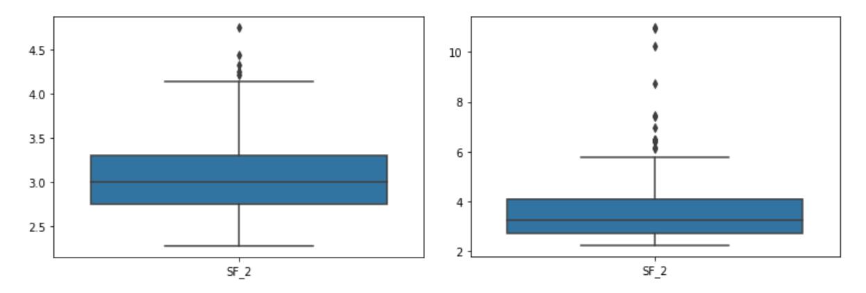
Figure 7 Box-plots of safety-factors F1 (left) and I0 (right).
Statistics F1 Safety Factor I0 Safety Factor Mean 3.057512 3.659426 Std. 0.452896 1.428222 Min 2.28 2.23 25% 2.75 2.71 50% 3.01 3.25 75% 3.31 4.07
Table 8 Statistic description of the safety factors of F1 and I0.
In general, both models showed that areas of intact pillar stability may contain failed pillars. This result confirms our suspicion of the existence of pillars with the potential to be dangerous despite their theoretically high safety factors.
Max 4.75 10.98
Conclusions
This study successfully obtained four new categories of pillar stability areas in coal mines using ANN-BP. The stability areas in these four new categories were successfully classified using a multiclass SVM. The process has two stages, starting with the process of determining new data classification using the ensemble learning ANN-BP with the ReLU, ELU, and GeLU activation functions, followed by the process of classifying areas of coal mine pillar stability using the multiclass SVM model with the kernel polynomial and RBF. It was implemented on four data proportions. Based on the results of ten experiments, the ensemble learning ANN-BP method could predict all four categories very well with an average accuracy of 92.98% and an accuracy standard deviation of 0.56%- 1.64%. Moreover, the classification process for areas of pillar stability using the multiclass SVM method with polynomial kernel and RBF kernel function had an accuracy of 91% and 92%, respectively. The multiclass SVM method with the RBF kernel function captured 96.6% of the F1 pillars, which have the potential to be dangerous at some point. The visualization results of the classification of areas of pillar stability showed that areas with intact pillars may also have failed pillars. These results also confirm our suspicion of the existence of pillars with the potential to be dangerous despite their theoretically high safety factors.
Acknowledgment
This study was funded by FMIPA Universitas Indonesia with assignment research grant scheme, 2022 (ID: 003/UN2.F3.D/PPM.00.02/2022).