
Introduction
Rainfall distribution is a crucial aspect of understanding hydrological cycles and their impact on various environmental processes. The spatial and temporal variability of rainfall plays a significant role in determining the characteristics and patterns of rainfall distribution. Studies have shown that rainfall is not uniformly distributed in space and time, and its distribution can vary across different regions and seasons [1]. The analysis of rainfall variability helps to understand the behavior of precipitation and its impact on various hydrological processes. Rainfall patterns in Malaysia and Indonesia are influenced by various factors, including the Asian winter monsoon and monsoonal winds [2, 3]. In Peninsular Malaysia and Indonesia, rainfall is more prevalent during the boreal winter, with the highest amounts observed along the east coast of Peninsular Malaysia, regions of Sumatra and Java, the northwest coast of Borneo, and the east coast of the Philippines [3]. The climatology of rainfall in Indonesia is like that of Malaysia, with both countries experiencing high rainfall rates during the same periods [4].
Copyright ©2024 Published by IRCS - ITB J. Eng. Technol. Sci. Vol. 56, No. 2, 2024, 287-303
Monsoon phenomena in Malaysia, particularly in Peninsular Malaysia, are influenced by various factors, such as regional wind flows, Indian Ocean variability, and global climate patterns [5]. The climate of Peninsular Malaysia is characterized by two main monsoon seasons, the Northeast Monsoon (NEM) and the Southwest Monsoon (SWM) [5]. The Northeast Monsoon occurs from November to March and brings heavy rainfall to the east coast of Peninsular Malaysia, making it highly susceptible to flooding and freshwater runoff [6]. On the other hand, the Southwest Monsoon occurs from May to September and affects the west coast of Malaysia [7]. Understanding the significant parameters contributing to the classification of precipitation is essential for accurate analysis and forecasting. Predicting rainfall has become increasingly important due to its impact on various sectors, such as agriculture [8], aquaculture [9], and the economy [10]. Factors such as the area where rainfall occurs, global heat, and indirect parameters associated with rainfall make it necessary to effectively predict rainfall from satellite images [11]. Therefore, developing rainfall prediction approaches that can determine when and what type of rain will occur is essential [12].
This study employed the Mahalanobis-Taguchi System (MTS) to classify and optimize the collected parameters to identify the significant parameters. MTS is a powerful algorithm [21] that combines Mahalanobis distance (MD) with Taguchi's method for pattern recognition [23], classification, optimization [22] and decision-making. It has been widely used in various fields, such as imbalance data classification [13], quality inspection [14], decision-making [15], feature selection [16], gait analysis [17], anomaly detection [18], bug fixing process management [19], quality classification [20], and many others.
Methodology
Figure 1 shows a concept flowchart of this study. This research utilized a Vantage Pro2 weather station, which was set up on UMPSA Pekan campus, Pahang, Malaysia. The weather station was primarily used to collect various parameter data. The data were collected every 30 minutes and stored in the weather station console. Table 1 shows 9 the identified parameters after the data was pre-processed.
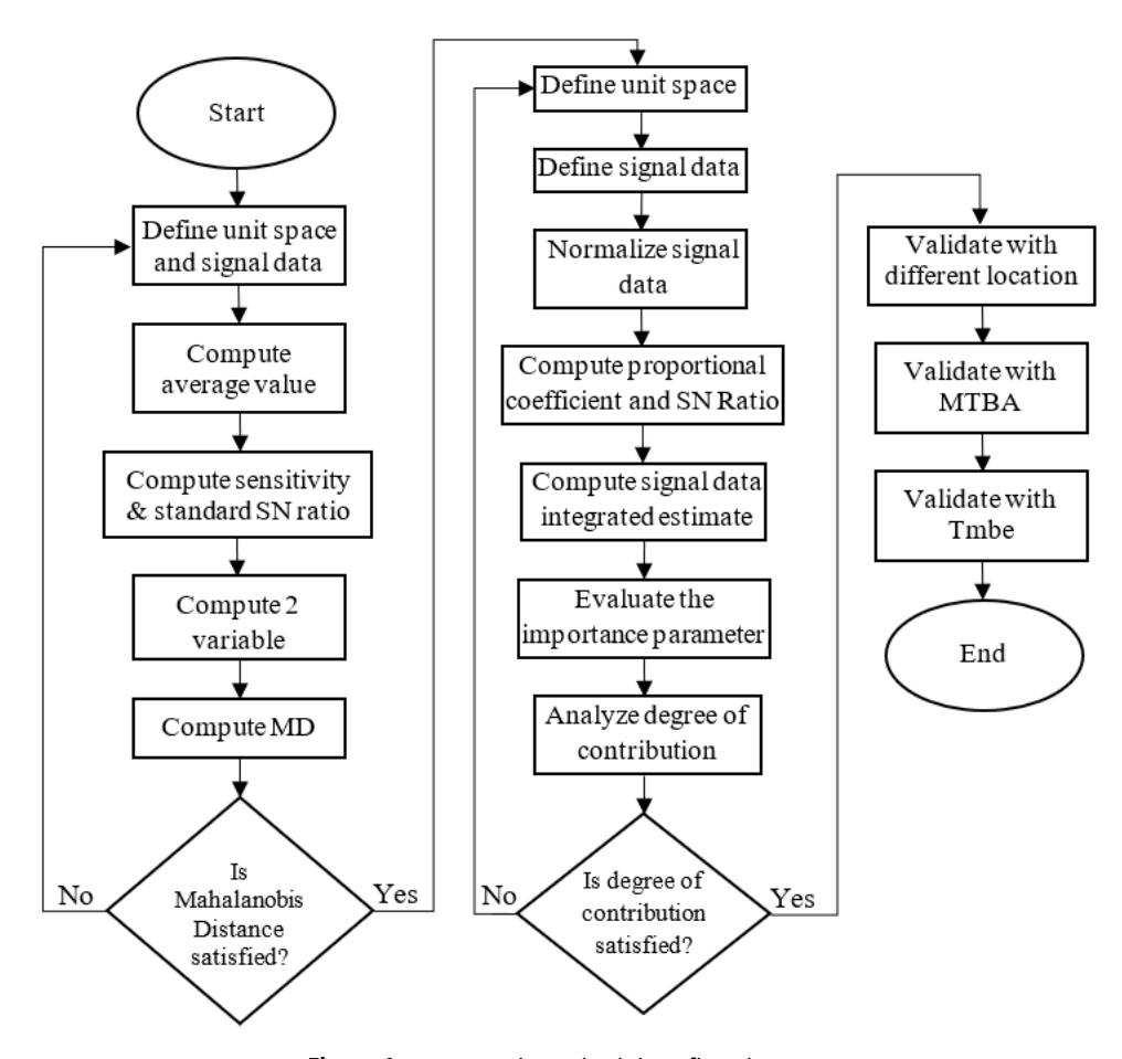
Research methodology flowchart.
| Numbers | Parameters/variables | Unit |
|---|---|---|
| 1 | Outside temperature | ℃ |
| 2 | High temperature | ℃ |
| 3 | Low temperature | ℃ |
| 4 | Outside humidity | ℃ |
| 5 | Dew point | ℃ |
| 6 | Heat index | - |
| 7 | Rain | mm |
| 8 | Rain rate | mm/hr |
| 9 | Cool degree-day | ℃ |
Table 1 Parameters/variables.
The RT method is used for the purpose of categorization due to its ability to categorize the parameters into two separate variables. In this study, the RT method provided the conceptual framework for defining the unit space and signal data in relation to precipitation. The unit space represents the absence of rainfall, while the signal data corresponds to the presence of rainfall. The average value for each parameter within the unit space is computed using Eq. (1).
\[\bar{x}_j = \frac{1}{n} (x_{1j} + x_{2j} + \dots + x_{nj}) \tag{1}\]
The sensitivity, β, the linear formula, L, and the effective divider, r, are computed by Eqs. (2) to (4) respectively.
Sensitivity, \[\beta_1 = \frac{L_1}{r}\] (2)
Linear equation, \[L_1 = \bar{x}_1 x_{11} + \bar{x}_2 x_{12} + \dots + \bar{x}_k x_{1k}\] (3)
Effective divider, \[r = \bar{x}_1^2 + \bar{x}_2^2 + \dots + \bar{x}_k^2\] (4)
Then, the total variations ST, variation of proportional term Sβ, error variation Se, and error variance Vel, are computed as shown in Eqs. (5) to (8) respectively.
Total variation, \[S_{T1} = x_{11}^2 + x_{12}^2 + \dots + x_{1k}^2\] (5)
Variation of proportional term, \[S_{\beta 1} = \frac{{L_1}^2}{r}\] (6)
Error variation, \[S_{el} = S_{T1} - S_{\beta 1}\] (7)
Error variance, \[V_{el} = \frac{S_{el}}{k-1}\] (8)
The computation of the standard signal-to-noise ratio (SNR) η1 is performed according to Eq. (9). As the value of η1 increases, the correlation between the input and the output increases.
Standard SNR, \[\eta_1 = \frac{1}{V_{e_1}}\] (9)
The computation of two variables, Y1 and Y2 , are computed by the sensitivity β standard SNR η using Eqs. (10) and (11).
\[Y_{i1} = \beta_i \ (i = 1, 2, ..., n)\] (10)
\[Y_{i2} = \frac{1}{\sqrt{\eta_i}} = \sqrt{V_{ei}} \ (i = 1, 2, ..., n) \tag{11}\]
Then, the means for Y1 and Y2 are computed for all the samples of the unit space as stated in Eqs. (12) and (13).
\[\bar{Y}_1 = \frac{1}{n}(Y_{11} + Y_{21} + \dots + Y_{n1}) \tag{12}\]
\[\bar{Y}_2 = \frac{1}{n} (Y_{12} + Y_{22} + \dots + Y_{n2}) \tag{13}\]
Finally, the Mahalanobis distances (MD) of the sample are calculated with Eq. (14).
Mahalanobis distance, \[D^2 = \frac{YA^{-1}Y^T}{k}\] (14)
For the signal data, the sensitivity β1 and the linear formula L ' are computed using Eqs. (2) and (3), and the effective divider r is used in the unit space. Then, the total variations ST, variation of proportional term Sβ, error variation Se, and error variance Vel, are computed through Eqs. (5) to (8) respectively. The value of sensitivity β and the standard SNR ŋ from the signal data are used for the computation of variables Y1 and Y2 as well. The value of sensitivity β is used for Y1 as stated in Eq. (10), while the variable Y2 is converted first as stated in Eq. (11) to allow the evaluation of scattering from the normal conditions. The average values for Y1 and Y2 are the same as shown in Eqs. (12) and (13), respectively, for the prediction of the healthy group origin. Lastly, the MD value is found based on the Eq. (14).
To optimize the data analysis, the T-Method 1 was used to compute the degree of contribution within the rainfall data set. The output value used in this study was determined by calculating the MD using the RT method. The average values for every parameter and the output average value from the samples were calculated as shown in Eqs. (15) and (16) respectively.
\[\bar{x}_j = \frac{1}{n} (x_{1j} + x_{2j} + \dots + x_{nj})\] (15)
\[\bar{y} = M_0 = \frac{1}{n} (x_{1j} + x_{2j} + \dots + x_{nj})\] (16)
The unit space was selected based on the average value for every parameter and the output. The unselected sample data were treated as signal data. After that the signal data sample were normalized as shown in Eqs. (17) and (18), respectively.
\[X_{ij} = x'_{ij} - \bar{x}_j \tag{17}\]
\[M_i = y'_{ij} - M_j \tag{18}\]
Then, proportional coefficient β and SNR ŋ were computed for each parameter as shown in Eqs. (19) to (25).
Proportional coefficient, \[\beta_1 = \frac{M_1 X_{11} + M_2 X_{21} + M_l X_{l1}}{r}\] (19)
\[SNR, \eta_1 = \begin{cases} \frac{\frac{1}{r}(S_{B1} - V_{e1})}{V_{el}} & (When S_{\beta 1} > V_{el}) \\ 0 & (When S_{\beta 1} < V_{el}) \end{cases}\] (20)
Effective divider, \[r = M_1^2 + M_2^2 + \dots + M_l^2\] (21)
Total variation, \[S_{T1} = X_{11}^2 + X_{21}^2 + \dots + X_{lk}^2\] (22)
Variation of proportional term, \[S_{\beta 1} = \frac{(M_1 X_{11} + M_2 X_{21} \cdots + M_l X_{l1})^2}{r}\] (23)
Error variation, \[S_{el} = S_{T1} - S_{\beta 1}\] (24)
Error variance, \[V_{el} = \frac{S_{el}}{l-1}\] (25)
After that, the integrated estimate value of signal data was computed by using proportional coefficient β and SNR η for each parameter, as shown in Eq. (26).
\[\widehat{M}_{i} = \frac{\eta_{1} \times \frac{X_{i1}}{\beta_{1}} \times \eta_{2} \times \frac{X_{i2}}{\beta_{2}} + \dots + \eta_{k} \times \frac{X_{ik}}{\beta_{ik}}}{\eta_{1} + \eta_{2} + \dots + \eta_{k}}\] (26)
Then, the integrated estimate SNR ŋ was computed using Eqs. (27) to (33):
Integrated SNR, \[\eta_1 = 10\log\left(\frac{\frac{1}{r}(S_{B1}-V_e)}{V_e}\right)\] (27)
Linear equation, \[L = M_1 \widehat{M}_1 + M_2 \widehat{M}_2 + \dots + M_l \widehat{M}_l\] (28)
Effective divider, \[r = M_1^2 + M_2^2 + \dots + M_l^2\] (29)
Total variation, \[S_T = \widehat{M}_1^2 + \widehat{M}_1^2 + \dots + \widehat{M}_1^2\] (30)
Variation of proportional term, = 2 (31)
Error variation, \[S_e = S_T - S_\beta\] (32)
Error variance, \[V_e = \frac{S_e}{l-1}\] (33)
The relative importance of a parameter was determined by the extent to which the estimated SNR degraded when the parameter was omitted. Level 1 and level 2 of the orthogonal array (OA) were utilized for evaluation purposes. Utilizing OA permits the estimation of the SNR under various conditions. The two-level OA indicates that level 1 is a parameter, whereas level 2 is not. The difference between the SNR averages for levels 1 and 2 for each parameter was used to ascertain the relative importance of the parameters in terms of the estimated SNR. The degree of contribution was computed using Eq. (34):
Degree of contribution = \[\overline{SNR}_{level-1} - \overline{SNR}_{level-2}\] (34)
Finally, the result was validated with a data set from a different location, and the Jaccard similarity coefficient was used to determine the similarity in the parameters between the two locations. In addition, the obtained results were further compared with the MTBA to identify the significant parameters. The SNR was used to compare the results. The last step involved comparing the obtained results with the T mean-based error (Tmbe) to ascertain the error trends within the data sets. The performance of measure was evaluated using mean absolute error (MEA) and root mean square error (RMSE).
Result and Discussion
RT Method
Scatter plots were constructed using the results obtained from the RT method, with a focus on analyzing the relationship between the variables in relation to the monsoon phenomena. The months were divided according to the monsoon phenomena. The following graphs illustrate the use of the RT method to generate variables Y1 and Y2, which represent the classification between the unit space and the signal data, respectively. Figure 2 displays a scatter plot illustrating the relationship between the rainfall data in the unit space and the signal data within the context of the Northeast Monsoon phenomenon. First of all, for November, the unit space had 1,270 samples, while the signal data had 170 samples. The maximum and minimum value of MD for the unit space were 20.8599 and 0.0025, respectively, while the signal data were 1,983.74 and 0.0066, respectively.
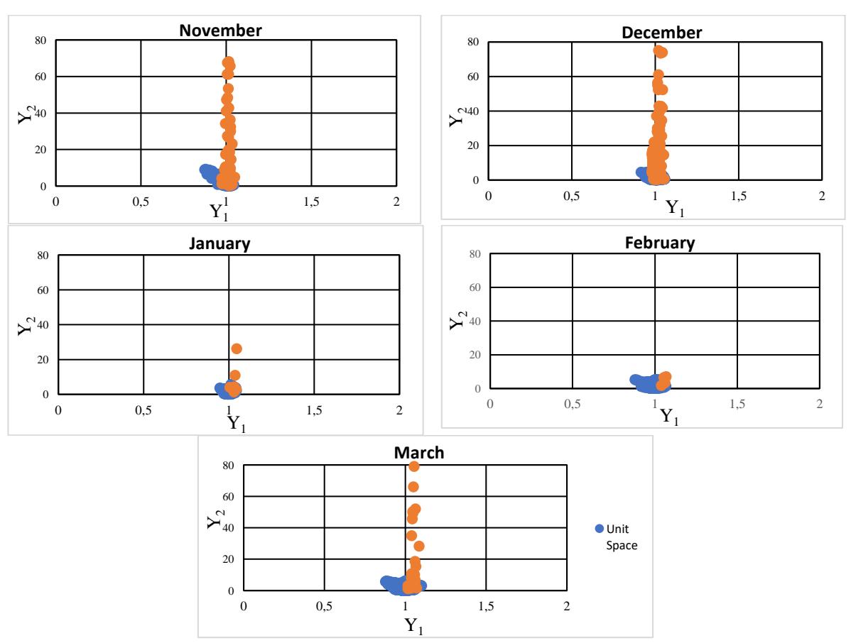
Scatter plot for the northeast monsoon phenomenon.
The average value of MD for the unit space was 1.0000 and 113.41 for the signal data. Next, the signal data for December had 178 samples, while the units space included 658 samples. The signal data were 2035.7 and 0.1120, while the maximum and minimum values of MD for the unit space were 7.4080 and 0.0055, respectively. The average MD value for the signal data was 119.5160 and 1.0000 for the unit space. In addition, for January, the unit space had 232 samples, while the signal data had 7 samples. The maximum and minimum value of MD for the unit space was 5.5620 and 0.0105, respectively, while for the signal data it was 166.1950 and 1.2276, respectively. The average value of MD for the unit space was 1.0000 and 28.5554 for the signal data. Moreover, while the signal data only had 4 samples for February, the unit space had a much higher number of samples i.e., 688. While the signal data were 11.5178 and 0.9391, respectively, the maximum and minimum values of MD for unit space are 10.7084 and 0.0072, respectively. The average MD value for the signal data was 6.0842 and 1.0000 for the unit space. Furthermore, the signal data for March had 32 samples, while the unit space had 1455 samples. The signal data are 27.3401 and 0.2668, respectively, the maximum and minimum values of MD for the unit space were 6.9994 and 0.00218, respectively. The average MD value for the unit space was 1.0000, and the average MD value for the signal data was 3663.1800. Therefore, the figure shows that the patterns were different from month to month due to the difference between normal and abnormal samples. The lower and upper MD values also have an effect on the patterns.
Figure 3 shows a scatter plot illustrating the relationship between rainfall in the unit space and the signal data during the Southwest Monsoon phenomenon. In the month of May, the unit space consisted of a total of 1,439 samples, while the signal data comprised only 46 samples. The highest and lowest values of MD for the unit space were 15.3683 and 0.2004, respectively. The corresponding signal data values were 1033.3416 and 0.0003, respectively. Besides, the mean value of MD for the unit space was 1.0000, while it was 89.6503 for the signal data. Other than that, the dataset for June consisted of 73 samples, while the total number of samples in the population was 1,366. The signal data consisted of two values, i.e., 2466.9000 and 0.0959.
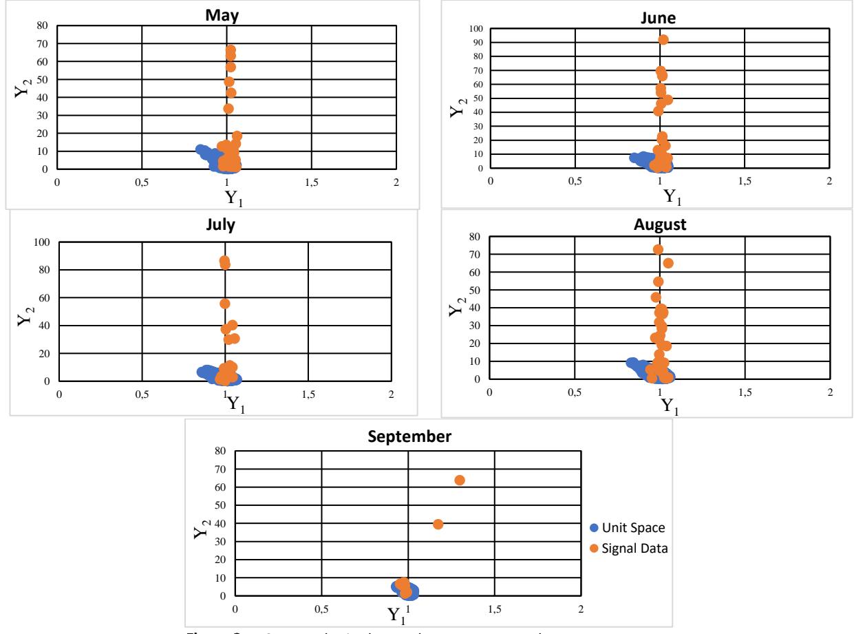
Figure 3 Scatter plot in the southwest monsoon phenomenon.
For the unit space, the maximum and lowest values of MD were 12.8708 and 0.000012, respectively. It is worth noting that the mean MD value for the signal data was 139.0290, while for the unit space it was 1.0000.
Nevertheless, for the month of July, the unit space had a total of 1457 samples, although the signal data consisted of only 30 samples. The MD values for the unit space ranged from a minimum of 0.0003 to a maximum of 8.7691. The signal data values ranged from a minimum of 0.2154 to a maximum of 2113.7535. The mean value of MD for the unit space was precisely 1.0000, while for the signal data it was 210.432. On the other hand, although the number of samples in the signal data for the month of August was limited to 56, the unit space had a much larger data set of 1,316 samples. The signal data comprised two values, namely 1444.9746 and 0.2730. Within the unit space, the highest and lowest values of MD were 15.6998 and 0.0005, respectively. It is worth noting that the mean MD value for the signal data was 130.691, while it was 1.0000 for the unit space. Lastly, for the month of September, the data set consisted of 21 samples, while the unit space data set contained 169 samples. The signal data consisted of 2 values, i.e., 7.2700 and 0.0447. In contrast, the highest and lowest values of MD for the unit space were 4.760 and 0.0060, respectively. The mean MD value for the signal data and the unit space was 1.000. As a result of the difference between normal and abnormal samples, the patterns varied from month to month, as can be seen in the figure. Besides, lower and higher MD values influenced the pattern.
It can be concluded that there was an overlap between the unit space and the signal data sample because the range number of MD for both samples overlapped with the maximum unit space and the minimum signal data. This system is still acceptable because the average of the signal data was not in the range of the unit space and the MD value will be used as output value for T-Method 1.
T-Method 1
The results for the T-Method 1 can be divided into three phenomena, i.e., the Northeast, the Southwest, and the Transition phase. To minimize computation, only the result for November is shown in this work. In Figure 4, the data are arranged in ascending order based on the MD value obtained by the RT technique. Subsequently, the average of all data and unit values were computed. The purpose of this stage was to determine an approximate function by using the unit space as the reference standard and the remaining data as signal data.
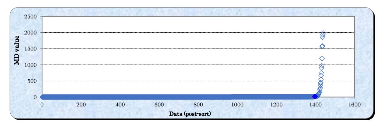
Graph of output value after sorting for November.
Figure 5 presents a scatter plot illustrating the relationship between the factors and their corresponding MD values for all nine parameters. In this stage, the proportional coefficient and signal-to-noise ratio (SNR) of each signal data were calculated by using the relationship between the MD value and the variable values. As the SNR increased, the correlation between the MD value and the value of the variables approached a linear relationship. The parameter rain rate exhibited the greatest SNR and a positive proportional coefficient, which supports the assumption that the rain rate is suitable for the overall goal of making general estimates. The SNR for the variable of high temperature exhibited the lowest value, making it less advantageous for general estimate purposes. Thus, the MD values of the nine parameters used showed different trends between P and SNR.
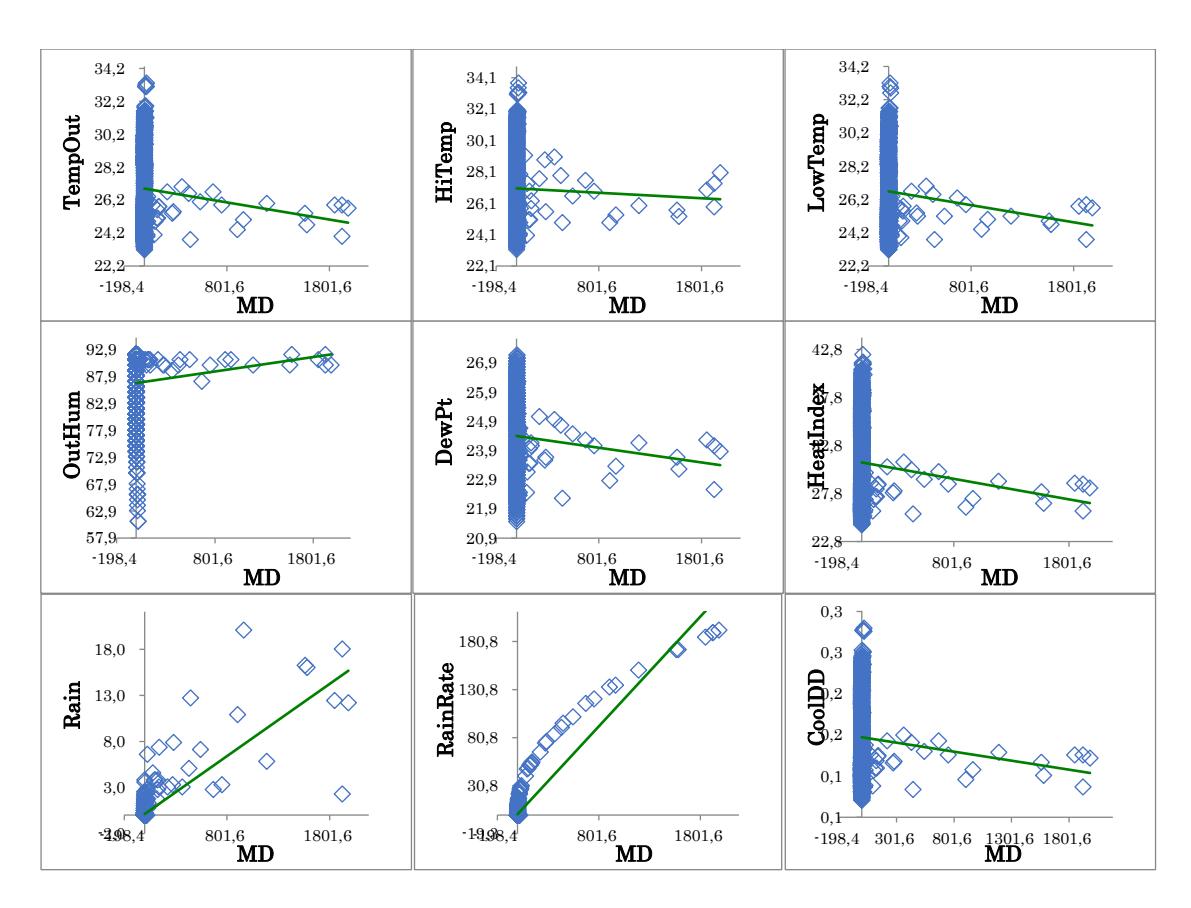
Figure 5 Scatter diagrams for relationship of input and output.
Figure 6 displays the outcome of the computational process for determining the estimated value \(\hat{M}\) of the signal data. The scatter diagram represents the relationship between the actual values, shown on the horizontal axis, and estimated values \(\hat{M}\), shown on the vertical axis. When the estimated values align with a linear trend, it suggests that a reliable estimation has been achieved. Moreover, the graph also exhibits the slope and the correlation coefficient.
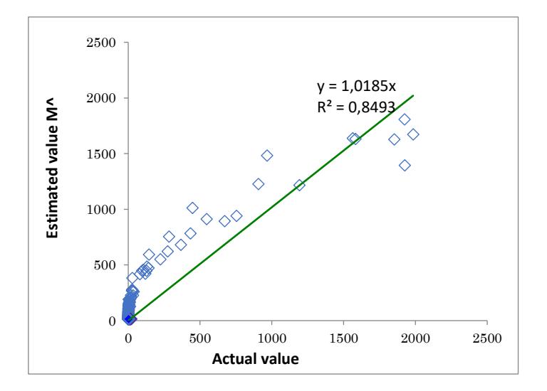
Figure 6 Distribution of actual and estimated values of signal data in November.
Table 2 in this work presents the integrated estimate of the SNR in decibels (db) for the auxiliary variables. The values in this table were derived by computing the SNR of the orthogonal array on a row-by-row basis. The degree of contribution was determined by calculating the SNR.
| Table 2 Integrated estimation of SNR (db) by parameter levels. |
|---|
| Parameter | Level 1 | Level 2 | Degree of contribution |
|---|---|---|---|
| Outside temperature (A) | -43.569 | -48.769 | 5.201 |
| High temperature (B) | -48.765 | -43.573 | -5.192 |
| Low temperature (C) | -49.932 | -42.406 | -7.526 |
| Outside humidity (D) | -43.568 | -48.77 | 5.203 |
| Dew point (E) | -42.42 | -49.918 | 7.499 |
| Heat index (F) | -49.939 | -42.399 | -7.540 |
| Rain (G) | -37.61 | -54.728 | 17.118 |
| Rain rate (H) | -34.67 | -57.668 | 22.998 |
| Cool degree-day (I) | -48.769 | -43.569 | -5.201 |
The factorial effect is graphed in Figure 7 by using the SNR across several levels. In the month of November, there was a decrease in many variables, such as outside temperature, outdoor humidity, dew point, rain, and rain rate, as shown by a descending trend in the respective SNRs broken line graph. These variables positively contributed to the estimated value, suggesting that using them may enhance the accuracy of the estimation. The use of factors such as high temperature, low temperature, heat index, and cool day degree has the potential to decrease the accuracy of the calculated values.
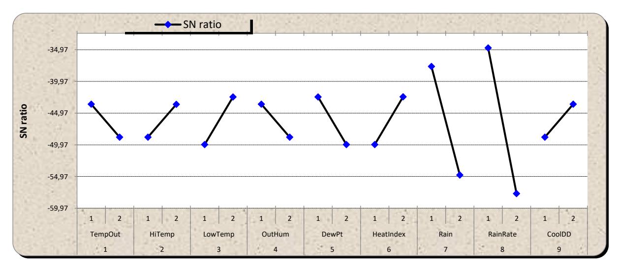
Factorial effects for November.
Subsequently, based on the factorial effect graph, a summary of the degree of contribution was created for all phenomena. Tables 3, 4, and 5 indicate the degree of contribution of all parameters for the Northwest Monsoon, the Southwest Monsoon, and the Transition Monsoon phenomenon, respectively.
Table 3 Summary of degree of contribution in the Northeast Monsoon phenomenon.
| Parameter | November | December | January | February | March |
|---|---|---|---|---|---|
| Outside temperature (A) | 5.201 | 3.007 | 3.379 | -0.111 | -0.442 |
| High temperature (B) | -5.192 | -3.329 | -3.241 | -1.131 | -0.610 |
| Low temperature (C) | -7.526 | -2.759 | -2.859 | -1.852 | -0.601 |
| Outside humidity (D) | 5.203 | 3.582 | 3.776 | 0.931 | -0.092 |
| Dew point (E) | 7.499 | 2.541 | 2.978 | 2.984 | -0.356 |
| Heat index (F) | -7.540 | -2.801 | -2.898 | -1.870 | -0.382 |
| Rain (G) | 1 7.118 | 10.270 | 8.644 | 3.149 | -0.132 |
| Rain rate (H) | 22.998 | 11.730 | 20.124 | 3.257 | 8.847 |
| Cool degree-day (I) | -5.201 | -3.548 | -3.220 | -1.239 | -0.560 |
| Parameter | May | June | July | August | September |
|---|---|---|---|---|---|
| Outside temperature (A) | 7.758 | 5.023 | 4.127 | 3.988 | 1.229 |
| High temperature (B) | -7.758 | -4.999 | -4.076 | -3.922 | -1.878 |
| Low temperature (C) | -5.121 | -5.820 | -5.141 | -5.033 | -2.390 |
| Outside humidity (D) | 7.758 | 5.005 | 4.016 | 3.722 | 1.399 |
| Dew point (E) | 5.121 | 5.794 | 5.145 | 4.936 | 1.701 |
| Heat index (F) | -5.124 | -5.841 | -5.171 | -5.045 | -2.373 |
| Rain (G) | 19.794 | 18.702 | 15.016 | 13.584 | 6.244 |
| Rain rate (H) | 30.320 | 16.729 | 15.050 | 14.648 | 6.043 |
| Cool degree-day (I) | -7.758 | -4.977 | -4.042 | -3.903 | -2.082 |
Table 4 Summary of degree of contribution in the Southwest Monsoon phenomenon.
Table 5 Summary of degree of contribution in the Transition Monsoon phenomenon.
| Parameter | April | June |
|---|---|---|
| Outside temperature (A) | 2.973 | 4.751 |
| High temperature (B) | -3.160 | -4.739 |
| Low temperature (C) | -3.678 | -6.1868 |
| Outside humidity (D) | 2.891 | 4.707 |
| Dew point (E) | 3.604 | 6.163 |
| Heat index (F) | -3.748 | -6.205 |
| Rain (G) | 8.824 | 15.082 |
| Rain rate (H) | 15.793 | 18.009 |
| Cool degree-day (I) | -3.258 | -4.740 |
In the context of MTS, there were three potential outcomes for each parameter based on their degree of contribution. When the degree of contribution decreased from left to right or exhibited a positive trend (green color), the utilization of these parameters resulted in an increase in the estimated value. Therefore, it is advisable to include these parameters, as they can enhance sensitivity and accuracy. On the contrary, when considering a decrease in the degree of contribution or a negative impact (red color), the use of these parameters resulted in a reduction of the estimated value. These parameters may be removed from the analysis, as they do not have a significant influence on sensitivity and accuracy. In addition, it is essential to avoid negative degrees of contribution since they have the potential to diminish both the sensitivity and the accuracy.
Validation
Validation with Different Locations
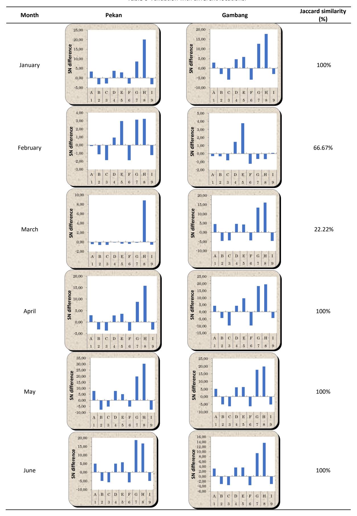
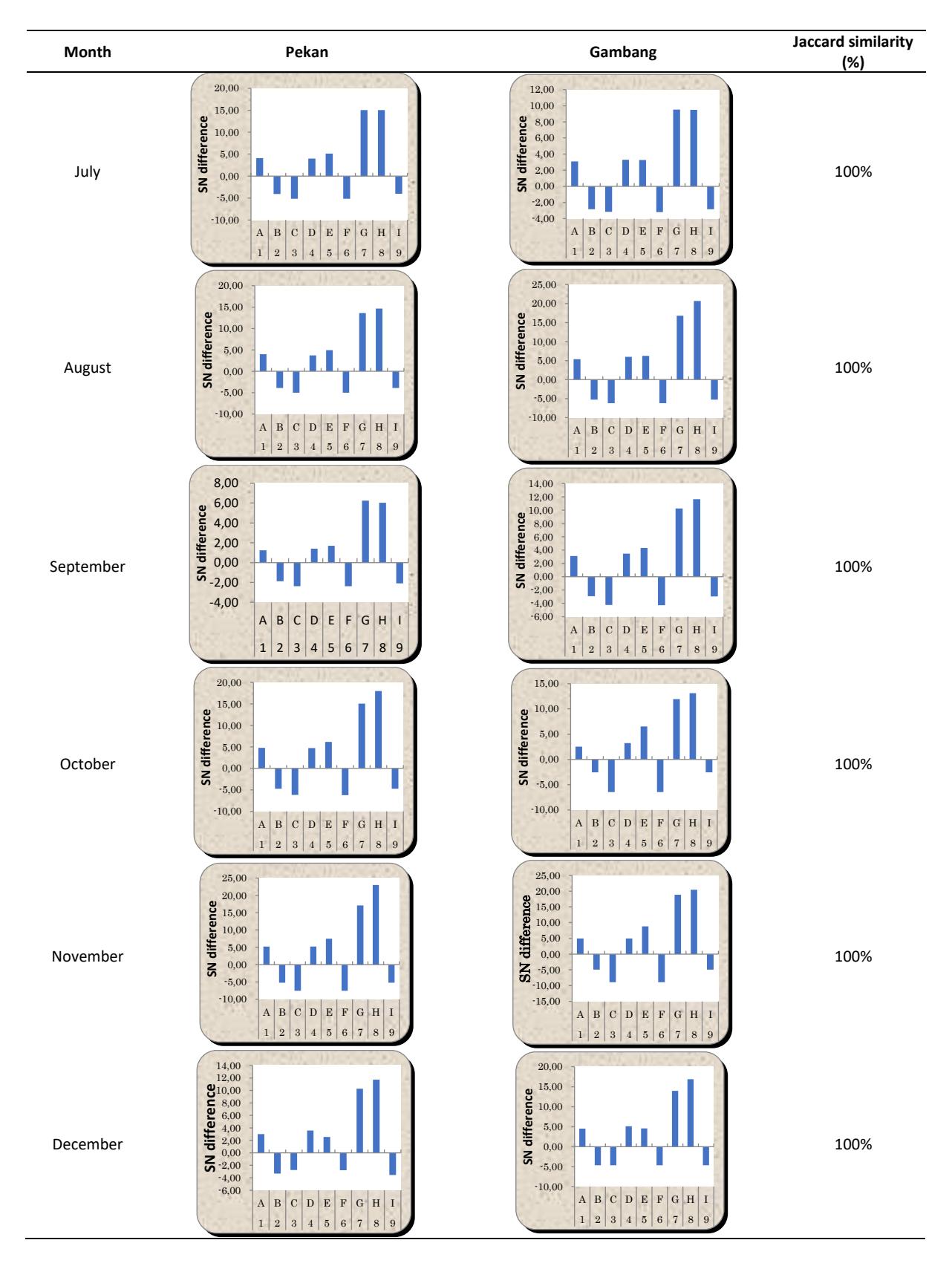
The location selected for the validation was the UMP Gambang campus, where identical devices were utilized as at the UMP Pekan campus. A bar graph for each month was constructed from the degree of contribution result. The Jaccard similarity percentage for January was determined by dividing the number of positive and negative bar similarities to Pekan (9 parameters) by the total number of parameters (9 parameters), and then multiplying the result by 100%.
The resulting similarity percentage was 100%. In February, the proportion of positive and negative bars comparable to Pekan (6 parameters) was calculated by dividing it by the entire number of parameters (9 parameters) and multiplying the result by 100%. The resulting similarity percentage was 66.67%. The parameters included in this calculation were outside temperature, rain, rain rate, and cool degree day. In the month of March, the ratio of positive and negative bars, like in Pekan, was calculated by dividing the number of similar parameters (2 parameters) by the total number of parameters (9 parameters).
This ratio was then multiplied by 100% to get the similarity percentage, which was found to be 22.22%. The two similar parameters in question were heat index and rain rate. Based on the similarity, it can be concluded that for March significant parameters were outside temperature, outside humidity, dew point, rain, and rain rate because of the similarity with significant parameters in Gambang campus except for February and March.
Table 6 Validation with different locations.
Validation with MTBA
In this section, as shown in Table 7, the SNR and significant parameters from MTS (Teshima) were compared with MTBA. For SNR, the gain was calculated by subtracting the SNR value after and before optimizing when the parameters were used. According to results of all the gain values, the MTBA values were higher than the MTS (Teshima) values because MTBA is a new enhancement method-based MTS. In terms of significant parameters, the parameters given by MTBA are a subset of those of MTS (Teshima). This means that MTBA can better optimize the parameters to get the significant parameters, as the gain is higher than with MTS (Teshima). For March, the gain was negative, as the rain rate is not the only significant parameter, but the parameters are still a subset of MTBA's significant parameters.
Table 7 Comparison of SNR results between MTS and MTBA.
| Month | Method | Significant parameters | SNR | Gain | |
|---|---|---|---|---|---|
| MTS (Jugulum) | All | 17.11 | N/A | ||
| 1. | January | MTS (Teshima) | A D E G H | 19.07 | 1.96 |
| MTBA | G H | 22.58 | 5.47 | ||
| MTS (Jugulum) | All | 13.86 | N/A | ||
| 2. | February | MTS (Teshima) | D E G H | 17.28 | 3.42 |
| MTBA | G H | 20.18 | 6.32 | ||
| MTS (Jugulum) | All | 14.61 | N/A | ||
| 3. | March | MTS (Teshima) | H | 10.98 | -3.63 |
| MTBA | G H | 20.57 | 5.96 | ||
| MTS (Jugulum) | All | 13.49 | N/A | ||
| 4. | April | MTS (Teshima) | A D E G H | 15.55 | 2.06 |
| MTBA | G H | 19.33 | 5.84 | ||
| MTS (Jugulum) | All | 12.35 | N/A | ||
| 5. | May | MTS (Teshima) | A D E G H | 14.42 | 2.07 |
| MTBA | G H | 18.16 | 5.81 | ||
| MTS (Jugulum) | All | 11.93 | N/A | ||
| 6. | June | MTS (Teshima) | A D E G H | 14.21 | 2.28 |
| MTBA | G H | 17.99 | 6.06 | ||
| MTS (Jugulum) | All | 12.34 | N/A | ||
| 7. | July | MTS (Teshima) | A D E G H | 14.39 | 2.05 |
| MTBA | G H | 18.14 | 5.8 | ||
| MTS (Jugulum) | All | 16.24 | N/A | ||
| 8. | August | MTS (Teshima) | A D E G H | 18.2 | 1.96 |
| MTBA | G H | 21.92 | 5.68 | ||
| MTS (Jugulum) | All | 15.84 | N/A | ||
| 9. | September | MTS (Teshima) | A D E G H | 18.23 | 2.39 |
| MTBA | E G H | 20.17 | 4.33 | ||
| MTS (Jugulum) | All | 14.46 | N/A | ||
| 10. | October | MTS (Teshima) | A D E G H | 16.63 | 2.17 |
| MTBA | G H | 20.43 | 5.97 | ||
| MTS (Jugulum) | All | 14.26 | N/A | ||
| 11. | November | MTS (Teshima) | A D E G H | 16.47 | 2.21 |
| MTBA | G H | 20.28 | 6.02 | ||
| MTS (Jugulum) | All | 14.51 | N/A | ||
| 12. | December | MTS (Teshima) | A D E G H | 16.75 | 2.24 |
| MTBA | G H | 20.5 | 5.99 |
Validation with Tmbe
In this stage, the model's effectiveness was assessed by randomly partitioning the data into training, testing, and validation sets for each month. The proportion of data allocated for validation purposes was 30% of the total data. The remaining data were divided into two sets, with 70% allocated for training and 30% for testing. Randomization is often used during partitioning to maintain data integrity and mitigate bias. This methodology guarantees that the samples are dispersed in a random manner throughout the sets, hence reducing any inherent patterns or sequencing in the data. By randomizing the data set prior to partitioning, the resultant subsets exhibit more representativeness and mitigate the potential bias of the model towards any one sequence or pattern.
The mean absolute error (MAE) and root mean square error (RMSE) were computed for each month. According to the data shown in Figure 8, the month of March exhibited the largest MAE values compared to the other months. Specifically, the recorded MAE for training, testing, and validation was 29.062, 36.804, and 90.907, respectively. In the meantime, the training dataset exhibited the lowest value of 0.699, while the testing data
set demonstrated a slightly higher value of 0.7218 for the month of February. Conversely, the validation data set showcases its lowest value at 0.6474 for the month of September.
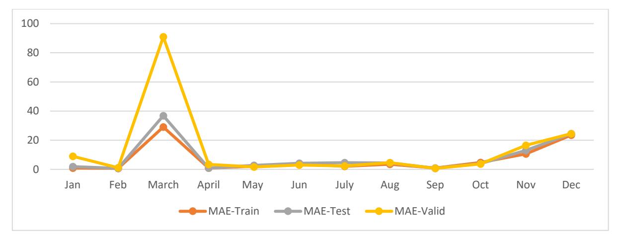
MAE of Tmbe.
Figure 9 shows the RSME values in relation to the Tmbe data. Specifically, the RSME values were the highest in March, which for training and testing were recorded as 283.04 and 352.04, respectively. The minimum values were observed in February, at 1.1502 for the training dataset and 1.1461 for the testing dataset.
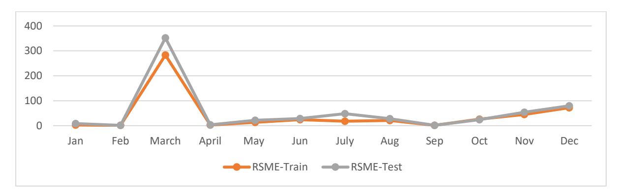
RSME of Tmbe.
Additionally, a comparison of the MAE results between Tmbe and T-Method 1 was conducted. The MAE training, testing and validation was performed for all months, as shown in Figure 10. According to the data shown in the figure, the MAE value for Tmbe was generally lower than the T-Method 1 in all months, except September. In September, the Tmbe values were 0.8741 for training and 0.8309 for testing. In the present study, the T-Method 1 yielded training and testing scores of 0.6804. Furthermore, in terms of validation, the recorded value for Tmbe in January was 8.9747, but the number for T-Method 1 was 1.8070. Based on the comparison, the significant parameters in March can be excluded from the final significant parameters, as the MAE values were higher for Tmbe and T-Method 1. This is because there were fewer significant parameters in March than in the other months. This will affect further predictions and increases the error. The month of March indicates that the model prediction was less accurate and the predictions were at a greater distance from the actual values. Then, the five significant parameters based on MTS from other months that could reduce the error for the prediction were outside temperature (A), outside humidity (D), dew point (F), rain (G) and rain rate (H).
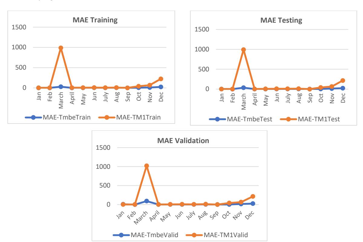
Comparison of MAE results between Tmbe and T-Method 1.
Conclusion
As the conclusion, MTS was able to classify the unit space and signal data using the RT method and determine the significant parameters for the rainfall trends data sets. Although the differences were small, the system seems acceptable because the average signal data did not fall within unit space. The significant parameters were used to assess each parameter's contribution using T-Method 1. A positive contribution determines each month's significant parameters. February had four Northeast Monsoon phenomenon parameters, while March had one, and November, December, and January each had five. There were five monthly parameters for the Southwest Monsoon phenomenon. The Transition Monsoon phenomenon had five significant parameters in April and October, the same as the Southwest Monsoon phenomenon. First, the significant parameters were validated using a dataset from the same type of weather stations with the same expectations but located in a different location. Other than February and March, most months had the same five significant parameters. Furthermore, the significant parameters were validated with MTBA using the SNR value. The gain for MTS (Teshima) was lower than for MTBA as the significant parameters were a subset of those of MTS (Teshima). Finally, validation with Tmbe showed that the MAE values were higher when compared to T-Method 1 for each month. The significant parametersin March can be excluded from the final significant parameters because Tmbe and T-Method 1 had higher MAEs, indicating that the model prediction was less accurate and the predictions was further from the actual values.
Acknowledgements
This research was fully supported by PGRS230320 and the authors fully acknowledge Universiti Malaysia Pahang Al-Sultan Abdullah for the approved fund that made this research viable and effective.