Introduction

The dynamics of fluid driven by gravity, frequently by variations in fluid density, is referred to as gravity current flow. This type of flow is prevalent in a variety of natural processes, such as the mixing of fluids in storage tanks, and industrial processes (Simpson, 1997) because of salinity differences (Garcia and Parsons, 1996) or variances in particle concentration (Necker et al., 2005). Foreseeing and managing the behavior of these systems requires an understanding of the dynamics of gravity current flow.

To gain understanding of the hydrodynamics of gravity currents, laboratory experiments are commonly carried out during both undergraduate and postgraduate studies. There are readily available teaching tools that allow for a relatively simple setup to investigate the flow. During these experiments dye is added to one of the fluids and the propagation of the flow is recorded by a camera. However, the only experimental results that can be obtained from these experiments are the location of the nose and the thickness of the head, and both are obtained only from visual interpretations of the data. The use of the light attenuation technique with the gravity current experiment requires a suitable light source and additional software for basic data analysis. Therefore, this method slightly increases the complexity of the experiments but at the same time, it enables a more rigorous definition of the location of the nose and the thickness of the head to be applied during the analysis of experimental data. It also allows for investigating the mixing characteristics of the two fluids in the highly turbulent layer immediately behind the current head.

In this study, a physical experiment was conducted in a teaching laboratory flume. Fresh water and sea water were poured into the flume with a gate separating the two fluids. The gate was opened to allow the fluids to flow by gravity. To contrast the motion of the two distinct fluids, dye was added to the lighter fluid. The light attenuation technique was utilized to capture the change in the light intensity as the flow travels passed. A separate calibration experiment was carried out to enable the decrease in the light intensity to be converted into the integrated salt concentration throughout the experiment. Due to the relatively short length of the teaching flume, this experiment only focuses on the initial phase of the gravity current, where the velocity is known to be almost constant. The results of the experiment

Copyright ©2025 Published by IRCS - ITB J. Eng. Technol. Sci. Vol. 57, No. 1, 2025, 118-128 ISSN: 2337-5779 DOI: 10.5614/j.eng.technol.sci.2025.57.1.9

revealed the dynamics of the flow and the mixing of the flow. A comparison with previously available data was carried out to assess the suitability of the light attenuation technique for investigating the gravity current flow.

This study enhances traditional gravity current experiments by incorporating the light attenuation technique, providing a quantitative approach to assess flow dynamics with greater precision. This method allows for a more nuanced investigation into the initial phase of gravity currents, facilitating a deeper understanding of mixing dynamics and offering a replicable model for future educational and experimental setups. The findings of this study contribute to advancing experimental methodologies for gravity current studies, particularly in controlled teaching environments, where the ability to measure flow mixing and turbulence with higher accuracy may offer new insights into the fundamental processes governing gravity-driven flows.

Experiment Methodology and Preparation

Light attenuation (LA) technique relates the decrease of light intensity to the increase of the concentration dye (mg/L) within the flume width. In other words, the light captured by a camera is brightest (i.e. highest light intensity) through clear water. As dye is added to the water, such as the red dye used in this study, the light captured by the camera becomes dimmer (i.e., a lower light intensity) as some of the light is attenuated. During a LA experiment, the light source is located on one side of the flume and the camera recording the light intensity is located on the other side. Therefore, the decrease in light intensity is related to the increase in the dye concentration integrated across the width of the flume. Dividing this integrated concentration (mg/l*m) by the width of the flume yields the average dye concentration across the flume. As red dye was added to the water, the decrease in the light intensity was based on the green part of the light spectrum. Calibration tests must be carried out to determine the relationship between the light intensity and the integrated dye concentration to yield the accurate results to be analyzed.

Throughout the experiment, 8-bit of light intensity was used. This system allows a range of light intensity from 0 to 255, with 0 being the darkest and 255 being the brightest. The camera used throughout this study is JAI AT-200 CL, which allows capturing of light intensity. The software used to analyze the light intensity is called Streams, a noncommercialized specially programmed software by Prof. Roger Nokes from the University of Canterbury, New Zealand (Nokes, 2005). The software can evaluate the green light intensity at any point of the image captured and return a numerical value. While this study made use of this specialized software, it is worth noting that the same tasks can be accomplished using relatively straightforward code in Python or MATLAB.

The description of the experiment set up is shown in Figure 1. First, the White LED Panel light source (manufactured by A&P Hong Kong Ltd., and consisting of 672 lamps each with a maximum power of 3 Watts) was put in place and turned on to provide a relatively white uniform background color. Then, the camera tripod was set up in place such that the flume was in between the light source and the camera (Figures 1 and 2).

Diagram of the experiment set up that involves the light source, flume, camera, and computer.

Photograph of the setup of the experiment that involves the light source, flume, camera, and computer.

The flume used in this experiment has typical dimensions for teaching flumes used for investigating the hydrodynamics of gravity currents. As such, this experiment will be easily reproducible for teaching purposes. Moreover, in this experiment, the effect of the distance between the light source and the flume or between the flume and the camera was negligible. The camera was set up to capture a significant portion of the flume and therefore was located sufficiently far away from the flume that the rays of light captured by the camera were close to parallel as they travelled through the flume, thereby avoiding parallax issues. Note that the preparation was done in an arbitrary light condition, but the calibration and the main experiment must be done in a dark room, enabling the LED panel to create a constant ambient light intensity to be captured by the camera. Lastly, the camera was connected to a computer with programs installed that control the camera, image capture and image analysis.

The following camera specifications were used throughout the calibration and the main experiment in this study:

• 1. Shutter Preset at 1/120,
• 2. Data capture setting was 8-bit, and
• 3. Auto-white-balance (AWB) was set to manual.
• 4. Pixel Depth at 8 (corresponding to 8-bit),
• 5. Horizontal dimension of 1616 pixels, and
• 6. Vertical dimension of 1236 pixels.

Special attention must be given to the maximum intensity captured by the camera. The aperture of the camera was adjusted so that the maximum intensity was just below 255. If by changing the aperture the intensities of the three colors were no longer similar, the auto-white-balance was pressed once more to reset the white balance.

Another important element of the preparation was to prepare the dye solution. Instead of adding a very small amount of dye powder every step, which was difficult to measure with the available measuring scale because of the very small amount of dye required, a better way was to prepare a dye solution at a certain constant concentration. In this experiment calibration, 30 mg/L concentration of dye was prepared, and at each step, 50 mL of this solution was poured into the tank. The Integrated Concentration of the solution was subsequently calculated post-experiment.

For the experiment itself, 10 L of fresh water was poured into the tank. The computer program Sapera Sequential Grab Demo was used to record the digital images of the data. The buffer was set to 50 frames. The captured image sequence was then saved as a video (.avi format) which was later separated into individual images using another program, VirtualDub. This procedure was repeated in every step. Note that in every step, 50 mL of the solution stated in the previous paragraph was added to the tank to increase the overall integrated concentration of the dye in the tank.

After all the images for the calibration were collected, Streams was used to conduct the analysis. For each image, the light intensity could be processed at different pixel locations. For the calibration, only the center pixel was used.

Because of the setup of the experiment, two calibrations were needed: (1) calibration to obtain the target dye concentration to ensure a linear relationship between integrated dye concentration and light intensity, and (2) the amount of crystalline sodium chloride used to artificially create unit weight of saltwater.

The calibration results for the relationship between the light intensity and Integrated Concentration are shown in Figure 3. As expected, the light intensity decreases when the Integrated Concentration of dye increases. The logarithmic ratio of the light intensity (LRLI) given by:

\[LRLI = ln\frac{I_0}{I} \tag{1}\] where is the green part of the light intensity in 8-bit while ⁰ is the initial 8-bit green light intensity when the dye concentration is 0 mg m/L.

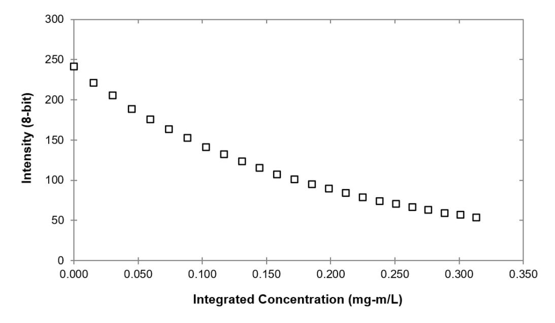
Calibration results showing intensity in terms of the amount of integrated dye concentration.

The relationship of LRLI versus the Integrated Concentration is plotted in Figure 4. This confirms the initial linear relationship between light intensity and the Integrated Concentration. However, for higher Integrated Concentration, the dye not only attenuates the light, but also starts to physically block the light. To obtain the maximum integrated concentration for which the linear relationship is appropriate, an error-analysis was conducted. A line was drawn between the origin and the maximum dye concentration so that the sum of the error between the real points and the estimated points was minimized. This analysis yielded the maximum Integrated Concentration that was used throughout the experiment of approximately 0.158 mg-m/L.

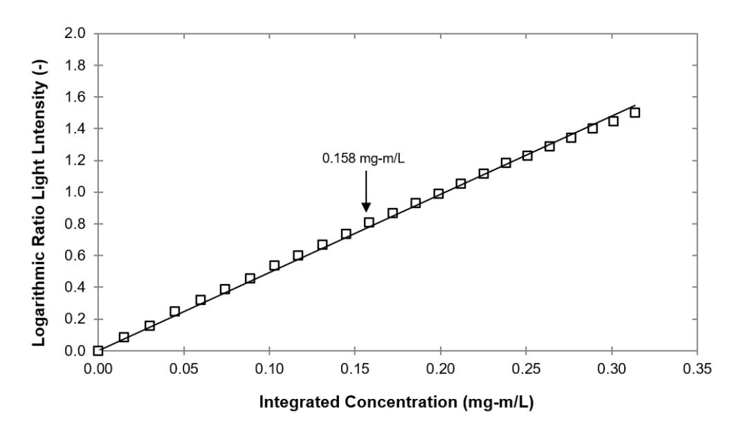
Calibration results showing LRLI in terms of the amount of integrated dye concentration.

Since the purpose of the study is to observe the gravity current between fresh water and salt water, the appropriate salt concentration was needed. A specific amount of crystalline sodium chloride was weighted and poured into the measuring cylinder filled with water that would be used for the experiment. Then, the mass of the solution was recorded for different concentrations. The relationship between the specific gravity of the solution and concentration of salt is depicted in Figure 5. Linear interpolation was utilized to find an approximation for the concentration of salt that yielded a solution with a specific gravity within the range of typical seawater (1.022-1.029). For example, a salt concentration of 50 mg/L yielded a specific gravity of 1.026 (dashed lines in Figure 5).

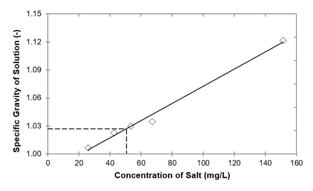
Relationship between the specific gravity of the solution and concentration of salt used.

Gravity Current Experiment and Observations

The overall set up during the calibration stage (Figures 1 and 2) was also adopted during the experiment. This included the preliminary preparations of the instruments used, the camera set up, and computer set up. Figure 6 illustrates the initial image being captured before and after dye concentration is added into the solution. Note that a gate was added to the flume to initially separate the two fluids of different density.

Based on the volume of water in the flume, the amount of crystalline salt added to the water was 1.1 kg and the amount of dye used was 28.5 mg. This yielded a specific gravity for the salt water of 1.023, which is within the range of typical seawater (1.022-1.029). In addition, the conversion length-scale between distances per pixel and per mm was determined to be 0.3490 mm/pixel. The camera then captured a sequence of 50 images as a background before both salt and dye were mixed inside. Another sequence of 50 images was captured for the red-dye calibration, after both salt and dye were mixed. Then, the gate was opened which generated the gravity current. The capturing technique recorded images at a frequency of 25 Hz with a total of 265 images per sequence. This captured the gravity current as it travelled from the gate to the opposite site of the field-of-view captured by the camera.

The initial condition of the flume before (a) and after (b) salt and dye were added, with the presence of a gate added to separate the two fluids.

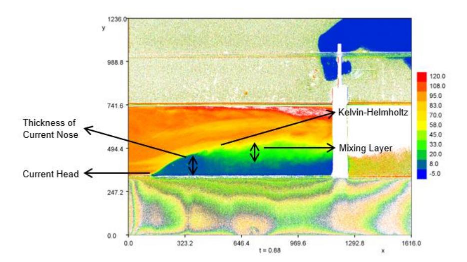
When the gate was removed, the denser fluid (saltwater) started to subduct and a current head (the nose-shaped interface between the two fluids) of the gravity current developed (Figure 7). Initially, or what we define as t = 0.0 s, we can observe the two fluids separated by the gate. As time progressed, the current consisted of dense fluid (clear saltwater) advancing along the bottom of the channel and the less dense fluid (red fresh water) flowing in the opposite direction on top of the dense fluid. From t = 1.2 to 6.0 s, we can see the current head of the dense fluid steadily progressing to the left of the image, below the less dense fluid. Behind the current head, the flow is turbulent. The high shear forces, due to the large velocity gradients caused by the two flows moving in opposite directions, subsequently results in significant mixing. This behavior is usually referred to as the Kelvin-Helmholtz instabilities. Due to the limited length of the flume, the current head hit the end of the flume and created some internal waves across the flume. The final results were the stratified layers of the salt water on the bottom, fresh water on top and a mixed layer of salt and fresh water observed in the middle.

Light Attenuation Technique Analysis of Gravity Current Experiment

The program Streams was used to analyze the results. An average image for both the water with zero dye (Background) and the water with the maximum Integrated Concentration of dye (Dye) were created by averaging the 50 images captured by the camera. Then, the two images were further processed by obtaining the LRLI in comparison with the Background. Thus, the Background image yielded zero everywhere while the Dye image yielded non-zero values (that varied based on the absolute light intensity). These two images were used to obtain the estimated Integrated Concentration at each time and pixel throughout the experiment, by linearly interpolating the LRLI between the zero and maximum Integrated Concentration. To aid the analysis of the mixing of the gravity current flow, Integrated Concentration results were generated that showed the variation in integrated concentration from 0 (salt water) to 100 (fresh water).

At this point, one might wonder why the hand and the gate are visible in all the Integrated Concentration images (Figure 7 (b) and (c)), but not in the actual images (Figure 7(a)). This is expected because the light attenuation technique compares the image at certain time with the Background image, which is in this case is associated with t = 0.0 s in Figure 7. The Background image includes the hand and the gate.

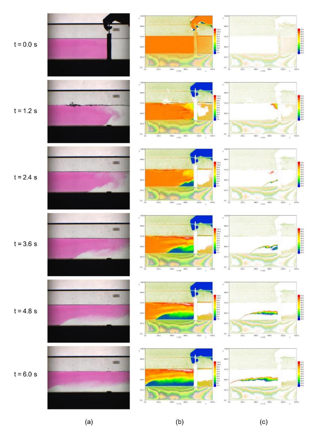
Time-series of the propagation of gravity current mixing with the colored images (a), overall Integrated Concentration Intensity (b), and Integrated Concentration Intensity of mixing layer thickness (c).

As part of undergraduate and postgraduate studies, the evolution of physical characteristics such as the location of the head and the nose thickness of the gravity current (Figure 8) are usually only estimated from the visual evidence (i.e., directly from images such as shown in Figure 7(a)). But the use of light attenuation technique allows these quantities to be defined in a more rigorous manner, using the integrated concentration results (Figure 7(b)). In this study, the location of the head was the distance above the bed where the Integrated Concentration was 50 (i.e., the middle of the interphase between the fresh and salt water).

Furthermore, while it is relatively straight forward to visually locate the head, precisely defining the thickness of the gravity current nose is usually a more difficult endeavor, since the region behind the head is unsteady and turbulent.

With the use of light attenuation technique, the thickness of the current nose could be defined as the location where the Integrated Concentration was 50 within a vertical cross-section (Figure 7(b)).

Using these definitions, the thickness of the head and the location of the nose were obtained from the experimental data. Starting from a time of 0.08 s, the thickness of the head, LH, grows and starting from a time of 2.4 s, it grows approximately linearly until a time of 3.6 s as shown in Figure 9. After that, the thickness of the head remains a relatively constant value of 50.1 mm with standard deviation of 1.1 mm (Figure 9). Comparing this value with the overall depth from the surface, which is H = 143.6 mm, the depth of the current head is estimated to be 0.35 H. This value is a little lower than the experiment done by Prastowo (2009) and Shin (2004) where the value obtained is between 0.36 H to 0.47 H (Prastowo, 2009).

Using the more rigorous estimations of the location of the nose of the gravity current, the velocity of the current was obtained by comparing its horizontal position in each subsequent frame to yield the distance travelled and then dividing by the time between frames of 0.04s. The velocity of the current head from 0.80 s to 4.80 s after the gate was lifted were obtained and the results are presented in Figure 10. The graph shows that the velocity was relatively constant within this time boundary, which matches previous results of the first phase of the gravity current (Kneller, Bennet, and McCaffrey, 1999, and Benjamin, 1968). The average constant current head velocity has been calculated to be 99.7 mm/s with a standard deviation of 5.8 mm/s.

Using the velocity estimates for the gravity current, the non-dimensional Froude (Fr) number can be found. The densimetric Fr equation is given by:

\[Fr = \frac{v}{\sqrt{\frac{(\rho - \rho_W)gL_T}{\rho_W}}} \tag{2}\] where is the velocity, is the acceleration of the salt water, is the density of the salt water, is the density of the fresh water, and is the total water depth. Though there are some deviations, the result obtained shows a nearly consistent value, which is directly related to the nearly constant values for the velocity and current head thickness. The average Fr number is 0.55, which is less than the general values between 0.7 and 1.4. The Fr number obtained in this study is less than the general values closer to 1 (Shin et al., 2004) or the theoretical value of 1.4 or √2 (von Karman, 1940). Even though the flow is driven by the density difference and hence the gravitational force. However, the friction force is not zero. Due to the small width of the flume, the friction force has a larger effect on the flow than for most gravity current experiments that are likely to have been carried out in wider flumes, resulting in a smaller velocity. At this point, the flow is very turbulent. This can be confirmed since the estimates for the velocity and thickness of the nose enable the Reynolds number (Re) of the gravity current to be determined. Re is given by:

\[Re = \frac{\rho v L_H}{\mu} \tag{3}\] where is the dynamic viscosity of the salt water and is the thickness of the current nose. Though there are some fluctuations, the time-series result obtained for Re is also nearly constant because the velocity and nose thickness are nearly constant within the timeframe of the experiment. The average Re number is 49,161. This confirms the visual observations that the flow behind the current head is very turbulent. The visual observations included the Kelvin-Helmholtz instabilities in the region behind the head of the gravity current that indicated the presence of the mixing layer generated by the two fluids travelling in opposite directions. The light attenuation technique also enables this more complex feature to be analyzed in some detail. The steepest gradient within a vertical profile of the integrated concentration results was found to be between the relative integrated concentrations of 30 to 70. Hence, the region with integrated concentration results in that range was defined as the mixing layer. Figure 7(c) presents the development of the mixing layer in terms of both shape and thickness against time, in particular from t = 3.6 to 6.0 s. Note that at a particular time, the thickness of the mixing layer is up to 0.25 H.

The final results, when the velocity of the flow in the flume has reached zero everywhere and hence the flow has reached a new stable equilibrium with a denser layer of salt water on the bottom and a less dense layer of fresh water at the top, are presented in Figure 11. The thickness of the final mixing layer is approximately 0.15 H. This is significantly less than the instantaneous thickness of the mixing layer, indicating that the duration of the strong mixing seen immediately behind the head of the gravity current was not sufficiently long to reach a state of permanent fully mixed fluids within the mixing layer.

Integrated Concentration Intensity image indicating the thickness of the gravity current nose.

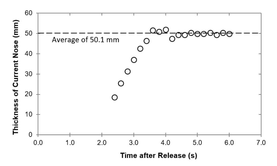
Evolution of the thickness of the current nose with time after gate release.

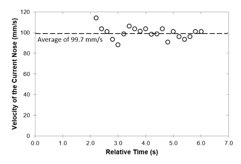
Evolution of velocity of the current nose with time after gate release.

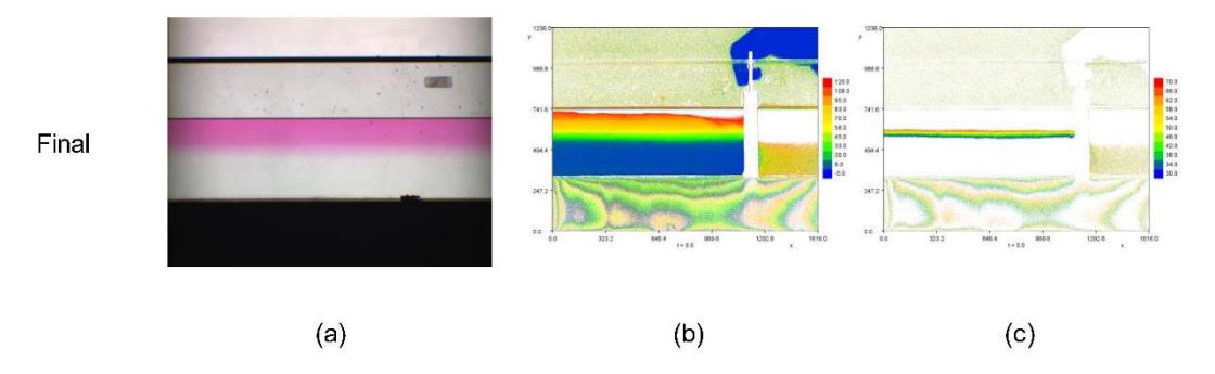
Final configuration of the gravity current mixing with the colored images (a), overall Integrated Concentration Intensity (b), and Integrated Concentration Intensity of mixing layer thickness (c).

Conclusion

The light attenuation flow visualization technique was used to obtain quantitative data from laboratory experiments of gravity currents generated in a simple uniform channel of constant width and depth. Gravity current experiments are commonly carried out as part of undergraduate and postgraduate studies, but generally only yield visual observations recorded by a camera. The use of light attenuation technique slightly increases the complexity of the experimental set up for the gravity current flow, as it requires a suitable light source and calibration of the dye, to determine the maximum integrated concentration and salt, to determine the density difference driving the gravity current to be added to the flume. In addition, it requires a calibration of the integrated concentration immediately before the experiment. The result from the light attenuation experiments then yield the integrated concentration field at each time interval that was converted into a relative salt concentration, between salt and fresh water.

Based on the results from the light attenuation experiments, a more rigorous definition of the location of the head and thickness of the nose of the gravity current were applied which also enabled the velocity the Froude number and Reynolds number of the current to be determined. Comparisons with previous experimental results showed that the data obtained using the light attenuation technique were within the expected range for a gravity current in a flume with a relatively small width. Behind the head of the gravity current is a region of high-turbulence and mixing of the salt and fresh water. Using the gradient in the integrated concentration field, estimates for the instantaneous and final thickness of the mixing layer were obtained, indicating that the duration of the strong mixing seen immediately behind the head of the gravity current was not sufficiently long to reach a state of permanent fully mixed fluids within the mixing layer.

The experimental data confirmed that the light attenuation technique can successfully be used to obtain detailed data of the hydrodynamics of the gravity current. And this is not limited to relatively small-scale experiments carried out as part of the current study. If a sufficiently large light source with a uniform light intensity is available, and there is space for the camera to be moved sufficiently far away from the flume so that parallax issues are mitigated, then the light attenuation technique can also be used to investigate large-scale flows. It is important however that these flows are essentially two-dimensional as the light attenuation technique yields the concentration integrated across the flume width.

Lastly, the use of light attenuation in this study advances the traditional approach to gravity current visualization by enabling a quantitative evaluation of flow characteristics, which opens avenues for more detailed analyses of mixing dynamics. This method provides an unprecedented look into the stratification and temporal evolution of mixing layers within gravity currents, underscoring its potential in both small-scale educational and larger-scale experimental applications. Future studies could adapt the light attenuation technique to explore large-scale gravity current flows by employing larger, uniform light sources, and ensuring camera placement that minimizes parallax effects. Investigating gravity currents across varying flume geometries, flow rates, and density gradients could further validate and expand the application of this method and ultimately enhance our understanding of mixing processes in both natural and industrial settings.

Acknowledgement

We would also like to thank Mr. Poon Man Fai and Mr. Fong Yiu Fai from the Hong Kong University of Science and Technology for their willingness and helpfulness with in-lab guidance and advice. We would like to specially thank Prof. Roger Nokes of University of Canterbury, New Zealand for allowing us to access Streams, a program used to conduct most of the analysis in this research work.

Compliance with Ethics Guidelines

The authors declare that they have no conflict of interest or financial conflicts to disclose.

This article does not contain any studies with human or animal subjects performed by any of the authors.