
Introduction
Buildings account for approximately 40% of the total global energy consumption (Jozi et al., 2022). Researchers are developing building energy management systems (BEMS) to manage energy demands and integrate renewable energy resources to minimize environmental impacts (Luo et al., 2020). The successful implementation of a BEMS requires accurate predictions of building energy consumption (Chou et al., 2017). Even a 1% improvement in the accuracy of energy consumption prediction can significantly enhance building energy efficiency (Weeraddana et al., 2021). However, forecasting building energy consumption remains a challenging task because of the dynamic nature of energy consumption, which changes over time (Jaramillo & Carrión, 2022). Forecasting encompasses not only energy consumption prediction, but also occupancy behavior and energy demand prediction, which are critical for optimizing systems such as HVAC (heating, ventilation, and air conditioning), lighting, windows, and charging stations, ultimately supporting demand-side management and balancing electricity markets. These interconnected aspects of prediction contribute to more effective energy planning, supply optimization, and efficient operation of BEMS (Li et al., 2024).
Energy consumption predictions can be divided into short-term (1 h to one week), medium-term (one month to one year), and long-term (more than one year) (Divina et al., 2018). Based on a literature review (Table 1), 83% of the reviewed studies focused on short-term energy consumption predictions. This is consistent with the findings of Kumar et al. (2024) who reported that 84% of studies focused on short-term forecasting, highlighting its dominance in the field. Short-term predictions provide BEMS with energy demand forecasts for scheduling power plant operations or
dispatching energy storage (Ji et al., 2022) and are vital for effective energy resource management (Luo et al., 2020; Somu et al., 2021). Therefore, this study focuses on the prediction of short-term building energy consumption.
| Ensemble Learning | _ | Weather Data | SWC | ıtext | ||||||
|---|---|---|---|---|---|---|---|---|---|---|
| Study | Bagging | Boosting | Stacking | Time Scope Horizon | Learning Method | Temperature | Humidity | Sliding Windows | COVID-19 Context | |
| (Somu et al., 2021) | - | - | - | Hourly | Building | CNN, LSTM | - | - | ٧ | - |
| (Weeraddana et al., 2021) | - | - | ٧ | Hourly | Nation | SVM, RF, LSTM, CNN, XGBoost | ٧ | - | ٧ | - |
| (Divina et al., 2018) | - | - | ٧ | Daily | Nation | RF, ANN | - | - | - | - |
| (Ji et al., 2022) | - | - | ٧ | Weekly, Monthly | Industry | GBDT, XGBoost, LightGBM | ٧ | ٧ | - | - |
| (Lee & Cho, 2022) | - | - | ٧ | Daily | Nation | SARIMAX, SVM, ANN | ٧ | ٧ | - | - |
| (K. Li et al., 2022) | - | - | ٧ | Hourly | Building | SVM, RF | ٧ | ٧ | - | - |
| (Wasesa et al., 2022) | - | ٧ | - | Daily | Building | SVM, XGboost, ARIMAX | - | ٧ | ||
| (Jaramillo & Carrión, 2022) | - | - | - | Monthly | City | ARIMA, ARMA | - | - | - | ٧ |
| (Saif et al., 2023) | ٧ | - | - | Daily | City | RF, KNN, PSO, SVM | ٧ | ٧ | - | ٧ |
| (Park et al., 2022) | - | - | ٧ | Hourly | Building | DNN, 1D CNN, LSTM | ٧ | ٧ | ٧ | - |
| (Cao et al., 2020) | ٧ | ٧ | - | Daily, Weekly | Building | SVR, XGBoost, RF | ٧ | ٧ | _ | - |
| (Vilaça et al., 2023) | - | - | - | Daily | City | LSTM-CNN | ٧ | ٧ | ٧ | ٧ |
| (Yu et al., 2021) | - | - | - | Daily | Nation | ResGCN | ٧ | - | ٧ | ٧ |
| This work | - | - | ٧ | Daily | Building | SVM, RF | ٧ | ٧ | ٧ | ٧ |
Table 1 Literature review of building energy consumption prediction studies.
The two approaches for obtaining energy consumption models are physics-based and data-driven. Physics-based models rely on analytical equations governed by physical laws, such as thermodynamics and heat transfer, to approximate the energy-consumption behavior of a building (Liu et al., 2019). Data-driven models utilize past energy consumption data to determine the relationship between the input variables (factors that affect energy consumption) and target variables (energy consumption) (Khairalla et al., 2018; Somu et al., 2021). This approach is more suitable for modeling complex systems. Developing a physics-based model from a complex system is time consuming, and some physical variables may not be available (Liu et al., 2019). Moreover, it is difficult to analytically model numerous interacting variables in a complex system, as in the present case. Data-driven models can infer patterns and predict building energy consumption more efficiently through training using historical data.
The data-driven approach relies on statistical techniques and machine learning (ML) algorithms to extract patterns and relationships from data. Statistical methods such as auto-regressive moving average (ARMA), auto-regressive integrated moving average (ARIMA) (Divina et al., 2018), seasonal ARIMA (SARIMA), exponential smoothing (Weeraddana et al., 2021), and SARIMA with exogenous variables (SARIMAX) utilize linear combinations of time-series components from the previous time step or seasonal component (Jaramillo & Carrión, 2022). Unfortunately, the models generated by these methods are only suitable for linear phenomena and their accuracy degrades when handling nonlinear dynamics (Khairalla et al., 2018). By contrast, ML methods have better capabilities and adaptations to nonlinear dynamics (Khairalla et al., 2018; Somu et al., 2021).
Recently, various ML methods have been utilized to predict building energy consumption. Moradzadeh et al. (2020) developed multilayer perceptron networks (MLP) and support vector regression (SVR) to model the cooling and heating loads of residential buildings. Ahmad et al. (2017) explored the performance of the random forest (RF) model in predicting building energy use (Ahmad et al., 2017). The study showed that the RF model achieved a performance on par with that of an artificial neural network (ANN). Wang et al. (2018) also reported the implementation of RF for energy-usage prediction (Wang et al., 2018). A comprehensive review of the ML methods used for energy consumption prediction is provided in Klyuev et al. (2022).
Although a single ML model predicts the energy consumption with satisfactory accuracy, the accuracy can be enhanced using the ensemble-learning (EL) method to combine multiple models (Divina et al., 2018; Weeraddana et al., 2021). A two-layer EL model was proposed by Divina et al. (2018). The bottom layer consisted of regression trees based on evolutionary algorithms, ANN, and RF, whereas the top layer consisted of generalized boosted regression models. Weeraddana et al. (2021) used a wide range of ML methods (tree-based models, deep learning models, and SVR) to create an EL model (Weeraddana et al., 2021). Both studies reported successful implementation of the EL method for energy consumption prediction.
In addition to the methods, the input variables for the models affect the prediction accuracy. Extreme weather conditions, special events, holidays, and pandemics may alter the usage patterns of building equipment, such as lighting and HVAC (Tomar et al., 2022; Weeraddana et al., 2021). These variables become inputs or features of ML models. Although adding more features can increase the accuracy of the model, it may also increase the complexity and computation time (Liu et al., 2022; Zhang & Wen, 2019). Therefore, feature selection is crucial as it contributes to the forecasting accuracy of the model.
Adding weather conditions as input variables can significantly improve the accuracy of energy consumption predictions (Lee & Cho, 2022). Temperature and humidity can influence thermal comfort inside buildings, which affects HVAC utilization. HVAC accounts for 40–60% of the energy usage in buildings (Asim et al., 2022). Extraordinary events such as the COVID-19 pandemic can disrupt energy consumption patterns. Previous research has incorporated Google Trends and Google Mobility (Wasesa et al., 2022) or lockdown policies (Arjomandi-Nezhad et al., 2022) as features to capture changing trends. However, these methods have high complexity and computational costs for accessing online data for real-time forecasting. Alternatively, sliding windows with a lower complexity can be used (Santos et al., 2021). This method uses previous energy consumption data to forecast future energy consumption (Chou et al., 2017). Incorporating recent observations with sliding windows enables the model to identify changes in patterns over time and improves its adaptability (Somu et al., 2021; Tomar et al., 2022).
Based on the literature review summarized in Error! Reference source not found., this study aims to develop an energy consumption model that can handle unexpected changes in energy consumption patterns by proposing a two-layer EL method. The adaptability of the model is enhanced by adding sliding windows as input features. Temperature and humidity are also added to account for the impact of weather conditions on energy consumption. Furthermore, investigating the influence of sliding windows as features for model adaptability and identifying the weather variables that have the most prominent impact on the prediction performance are among the objectives of this study. To evaluate the effectiveness of the proposed method, a model is deployed to forecast building energy consumption before (November 2019) and during (May 2020 - October 2020) the COVID-19 pandemic. The performance of the model is compared with that of a single ML model to demonstrate the relative performance of EL compared to the single SVR and RF methods. The contributions of this study, as highlighted in Table 1Error! Reference source not found., are as follows.
- 1. A novel approach is introduced that combines a two-layer stacking ML model with sliding windows as features and weather variables during the COVID-19 pandemic. The novelty of the method lies in exploring the use of sliding window features to enhance the adaptability of the model and identify the weather variables that most significantly impact prediction performance.
- 2. A model is proposed for predicting building energy consumption during the COVID-19 pandemic and its performance during the pre-pandemic and pandemic periods is compared. Most prior studies have focused on EL methods for specific applications, with limited attention paid to unexpected disruptions in energy consumption patterns during the COVID-19 pandemic.
The remainder of this paper is organized as follows: Section 2 describes the cross-industry standard process for data mining (CRISP-DM) framework used to develop the models. Section 3 discusses the results of the model deployment. Finally, Section 4 presents the main conclusions and explores potential future work.
Methodology
The CRISP-DM approach was adopted to develop the energy consumption models. CRISP-DM remains the de-facto standard in data-driven knowledge discovery and a commonly used frameworks for data mining (Ayele, 2020; Bošnjak et al., 2009; Martínez-Plumed et al., 2021; Schröer et al., 2021). It consists of six sequential steps: (1) business
understanding, (2) data understanding, (3) data preparation, (4) modeling, (5) evaluation, and (6) deployment. The implementation of CRISP-DM in this study is as follows.
Business Understanding
The objective of this study was to develop ML models for forecasting short-term (daily) building energy consumption to improve building energy management. The building under investigation was LABTEK XIX (latitude: -6.888340, longitude: 107.608565) at the Institut Teknologi Bandung, West Java, Indonesia. LABTEK XIX is a campus building that includes lecture halls, multimedia rooms, and a library. It has a total floor area of 5,430 m², six floors, a typical occupancy of 542 people, and an occupancy capacity of 775 people.
Data Understanding
Two data sources were available for modeling: (1) electricity data from intelligent power meters (PM2120) installed at the electrical panels of the building (Leksono et al., 2023) and (2) weather data from a Davis Vantage Pro automatic weather station (AWS), as shown in Figure 1. Figure 1 illustrates the data acquisition scheme.
(Automatic Weather Station) AWS DB Modelling Platform Power Meter DB
Intelligent Power Meter
AWS
Figure 1 Data acquisition scheme.
The building power consumption and weather data were sampled every 1 min and stored in a MySQL database, as summarized in Tables 2 and 3, respectively. The data types for each variable were integer (id, meter_id), datetime GMT+7 (timestamp), and float (Power, Voltage, Current, PF, F, Irradiance, Temperature, Wind Speed, Humidity). A total of 547,200 rows (data points) of raw data were collected. Raw data from the database were then pre-processed before being used as the training data.
| Table 2 | Examples of building energy consumption data during the observed tin | ne. |
|---|
| id | timestamp | meter_id | Power | PF | F | ||
|---|---|---|---|---|---|---|---|
| (kW) | (V) | (A) | (Hz) | ||||
| 7188905 | 2020-01-01 00:00:02 | 163 | 9.43 | 228.61 | 50.18 | 0.83 | 50.03 |
| 7188913 | 2020-01-01 00:01:03 | 163 | 9.23 | 228.70 | 50.01 | 0.81 | 50.04 |
| 7190089 | 2020-01-01 03:17:02 | 163 | 9.09 | 229.32 | 47.84 | 0.83 | 49.89 |
|---|---|---|---|---|---|---|---|
| 7190096 | 2020-01-01 03:18:02 | 163 | 9.34 | 229.25 | 48.64 | 0.84 | 49.87 |
| 7190102 | 2020-01-01 03:19:02 | 163 | 9.40 | 229.25 | 49.04 | 0.84 | 49.87 |
Table 3 Examples of weather data from the AWS during the observed time.
| timestamp | Irradiance (W/m²) | Temperature (°C) | Wind Speed (m/s) | Humidity (%) |
|---|---|---|---|---|
| 2020-05-22 09:01:00 | 308 | 24.7 | 0.4 | 87 |
| 2020-05-22 09:01:00 | 334 | 24.8 | 0.1 | 87 |
| 2020 03 22 03.01.00 | 334 | 24.0 | Ü | 07 |
| 2020-05-22 21:00:00 | O | 24.4 | O | 89 |
| 2020-05-22 21:00:00 | 0 | 24.4 | 0 | 89 |
| 0 | 0 | |||
| 2020-05-22 21:00:00 | 0 | 24.4 | 0 | 89 |
Data Preparation
In this step, the training datasets were prepared to develop the models. The target or output variable was daily energy consumption. Temporal features (day of year, day of week), sliding windows, temperature, and humidity were selected as the input variables. Temporal and sliding windows were generated based on the timestamp data. The daily energy consumption (in kWh) was calculated by summing the power consumption data (Figure 2) over a 1 d interval:
\[E = \frac{\sum_{t=0}^{t=1440} P_t \Delta_t}{60} \tag{1}\]
assuming constant power consumption during the sampling period. For temperature and humidity, the average values over 1 d were used (Figure 3). Subsequently, different input variables were combined to generate the following four datasets:
- 1. Group I: day of year, day of week, E<sub>day-1</sub>, E<sub>day-2</sub>, E<sub>day-3</sub>, E<sub>day-4</sub>, E<sub>day-5</sub>.
- 2. Group II: day of year, day of week, E<sub>day-1</sub>, E<sub>day-2</sub>, E<sub>day-3</sub>, E<sub>day-4</sub>, E<sub>day-5</sub>, temperature.
- 3. Group III: day of year, day of week, E<sub>day-1</sub>, E<sub>day-2</sub>, E<sub>day-3</sub>, E<sub>day-4</sub>, E<sub>day-5</sub>, humidity.
- 4. Group IV: day of year, day of week, Eday-1, Eday-2, Eday-3, Eday-4, Eday-5, temperature, humidity.
Eday-1 is a sliding window representing the energy consumption of the previous day, followed by Eday-2, Eday-3, Eday-4, and Eday-5, which represent the energy consumption of the earlier days. Sliding windows were generated by shifting the energy consumption data based on the timestamps. Before being used as training data, the datasets were scaled using the standard scaler technique to normalize the input data before being fed into the ML model.
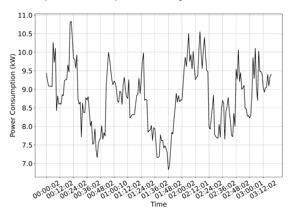
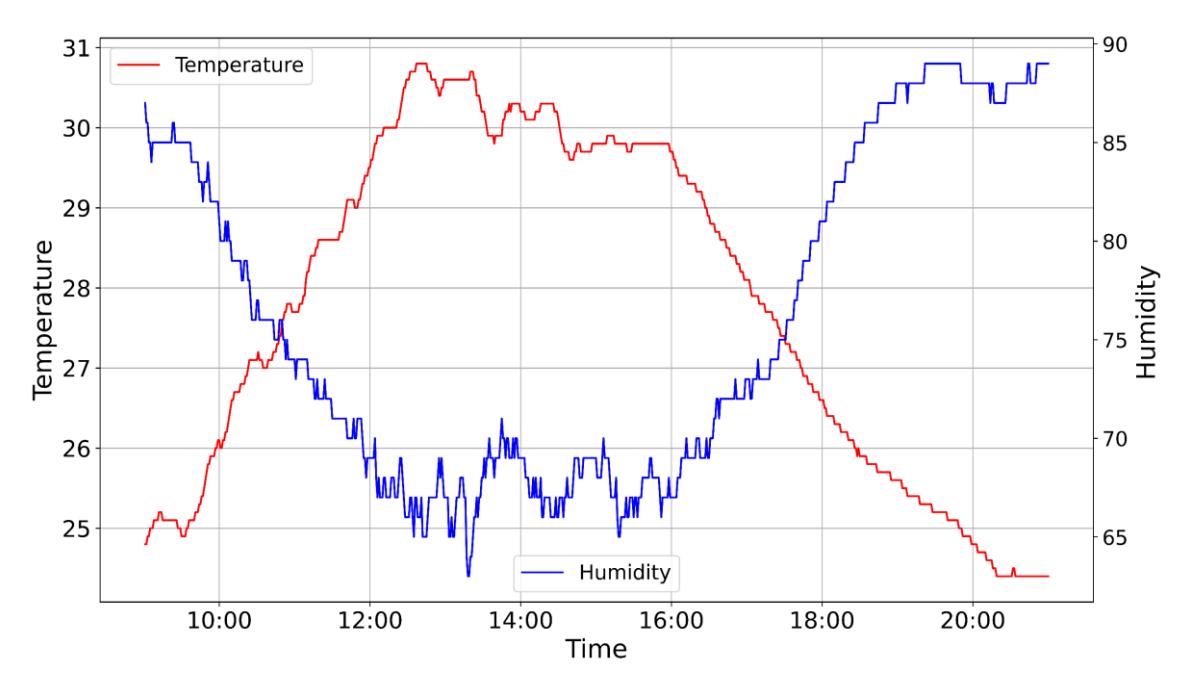
Figure 2 Examples of energy consumption data during the observed time.
Figure 3 Examples of temperature and humidity data during the observed time.
Modeling
The models were developed using two basic ML methods, SVR and RF, as well as the stacking EL method.
Support Vector Regression (SVR)
The main objective of SVR is to extract a regression function or model from time-series data that maps the input features to the target variable. The model is then used to forecast the future value of the target variable based on the available future input. By leveraging kernel functions, SVR can effectively find regression functions for input and output variables with a nonlinear relationship (Divina et al., 2018; Guo et al., 2021; Lee & Cho, 2022). Typical SVR training data for multiple input variables \(x_i\) and a single output variable \(y_i\) can be expressed as \((x_i, y_i)\), where \(x \in R^n\), i = 1, 2, ..., N, n is the dimension of input variables, and N is the number of training samples. The regression problem can be formulated as, \(y_i = f(x_i) = w \cdot \phi(x_i) + b\), where \(f(x_i)\) is the regression function, \(\phi(x_i)\) is a nonlinear mapping from the input space to a higher dimensional space, w is the weight, and b is a bias. Parameters w and b are obtained as follows:
\[\min \frac{1}{2} |w|^2 + C \sum_{i=1}^{N} \xi_i + \xi_i^*, \tag{2}\]
subject to \[\begin{cases} y_i - (\boldsymbol{w}^T + b) \le \varepsilon + \xi_i \\ (\boldsymbol{w}^T \boldsymbol{x}_i + b) - y_i \ge \varepsilon + \xi_i^* \\ \xi_i, \xi_i^* \ge 0 \end{cases}\] (3)
where \(\varepsilon\) is the error margin, C is a regularization parameter, and \(\xi\) is a slack variable. A detailed explanation of SVR is provided in (Lee & Cho, 2022; Wasesa et al., 2022).
Random Forest (RF)
RF is an aggregation of many decision trees (Breiman, 2001; Cha et al., 2021), each trained on a different randomly selected subset of the training data (Divina et al., 2018). It is essentially an ensemble of decision trees boosted by voting schemes to improve the predictive accuracy (Ahmad et al., 2017). Given \(X = x_1, x_2, ..., x_n\) as the N training data, where \(x_i\) is n-dimensional vector, RF generates several new training datasets through bootstrap sampling. Each dataset is used to grow decision trees \(T_1(X_1)\), \(T_2(X_2)\), ..., \(T_K(X_k)\) with outputs \(\hat{y}_1\), \(\hat{y}_2\), ..., \(\hat{y}_k\) respectively. RF produces only a single output. The final output \(\hat{y}\) is the average of all the individual tree outputs (Ahmad et al., 2017; Divina et al., 2018).
Ensemble Learning (EL)
The EL method addresses prediction problems by combining multiple ML models to improve accuracy compared with using individual models (Divina et al., 2018; K. Li et al., 2022). A formal derivation of the EL method is provided in (Hansen & Salamon, 1990). A two-layer stacking EL approach was employed in this study. Stacking combines several base models to produce the final predictions (Divina et al., 2018). In the first layer, SVR and RF models are used to estimate the target variable. Their outputs are then combined using linear regression in the second layer, as illustrated in Figure 4.
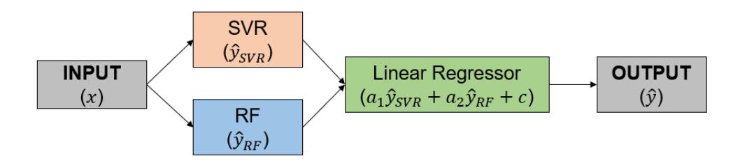
Figure 4 Two-layer stacking EL.
Six months (May 2019 – October 2019) of building energy consumption and weather data were used to train the models. As outlined in the data preparation step, there were four groups (Groups I– IV) in the datasets. Each method was trained on these datasets, resulting in a total of twelve models from a combination of the three learning methods and four datasets.
Evaluation
To evaluate the accuracy of each model, the performance was compared using three error metrics: (1) mean absolute error (MAE), (2) root mean square error (RMSE) and mean absolute percentage error (MAPE), as shown in Eq. (4). The prediction errors were calculated by comparing the predicted results \((\hat{y}_i)\) with the actual values \((y_i)\) for n data points or observations. Each of these metrics has distinct characteristics(Rai & Sahu, 2020). Combining these three metrics provides a better understanding of the model accuracy.
\[MAE = \frac{1}{n} \sum_{i=1}^{n} |y_i - \hat{y}_i|, \quad RMSE = \sqrt{\frac{1}{n} \sum_{i=1}^{n} (y_i - \hat{y}_i)^2}, \quad MAPE = \frac{1}{n} \sum_{i=1}^{n} \frac{|y_i - \hat{y}_i|}{y_i} \times 100\%.\] (4)
The MAE and RMSE were used to evaluate the 12 models obtained during the modeling step. Based on the evaluation results, the learning method that produced models with the highest accuracy was selected for deployment. The MAPE was used to compare the performance of the proposed methods with that of similar previous studies.
Deployment
In the deployment step, the models from the learning method selected in the previous step were used to predict the building energy consumption. The deployment was conducted under two conditions: before the COVID-19 pandemic (November 2019), when energy consumption was still high, and during the COVID-19 pandemic (May – October 2020) in Indonesia.
Results and Discussion
This section analyzes the models developed using the three different ML methods and four datasets. For the SVR model, an RBF kernel was used with C=9, \(\epsilon=0.01\), and \(\gamma=0.98\), while for the RF model, \(n\_estimator=99\). The hyperparameter settings for both the models were determined using the grid search method. To compare the performances of the models, each model was applied to predict the building energy consumption data for May–October 2019. Table 4 summarizes the prediction accuracy of each model based on the MAE and RMSE metrics. The EL model outperformed the other two methods, delivering better energy consumption predictions across all datasets (Groups I-IV). As expected, combining the two methods using an EL approach improved the prediction accuracy. Models trained with the Group III dataset were less accurate than those trained with Group I across all methods (SVR, RF, and EL), indicating that incorporating humidity into the Group I dataset did not improve the prediction accuracy. Based on the performance evaluation (Table 4), the EL model was selected and deployed to predict the daily energy consumption during both the pre-pandemic (November 2019) and pandemic (May - October 2020) periods.
| SVR | RF | EL | |||||
|---|---|---|---|---|---|---|---|
| Group | RMSE | MAE | RMSE | MAE | RMSE | MAE | |
| (kWh) | (kWh) | (kWh) | (kWh) | (kWh) | (kWh) | ||
| I | 67.92 | 11.00 | 38.76 | 8.04 | 4.65 | 2.76 | |
| II | 78.52 | 12.06 | 43.94 | 9.26 | 4.65 | 2.72 | |
| III | 87.88 | 14.18 | 50.62 | 9.52 | 4.92 | 3.05 | |
| IV | 80.61 | 12.65 | 40.31 | 8.65 | 4.25 | 2.61 | |
Table 4 Model performance on training datasets.
The pre-pandemic and training data had the same distribution, which was left-skewed (Figure 5), and exhibited similar variability, including a comparable range and interquartile range (IQR), as summarized in Table 5. This made it suitable for testing the EL models under pre-pandemic conditions. Figure 6 presents a sample of the actual and predicted results, and Table 6 summarizes the model performance for predicting pre-pandemic building energy consumption. Model performance was evaluated using the MAE, RMSE, and MAPE metrics. Among all the groups, Group II demonstrated the lowest error values, highlighting the significant role of temperature in improving the prediction accuracy. Temperature influences HVAC utilization, which, in turn, affects building energy consumption. However, the addition of temperature and humidity reduced the prediction accuracy, as observed in Group IV (MAPE = 4.20%). The performance decreased when only humidity was added, as in Group III (MAPE = 5.40%). Even the model trained with Group I (MAPE = 4.33%), which included only temporal features, performed better than that trained with Group III. These findings are consistent with those reported in Kelo & Dudul (2012).
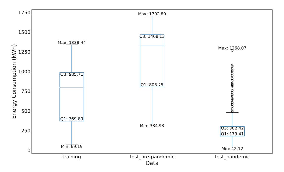
Box-plot comparison of energy consumption during pre-pandemic and pandemic periods.
| Statistical Parameter | Training Data (kWh) | Pre-Pandemic (kWh) | Pandemic (kWh) | Reduction* |
|---|---|---|---|---|
| Mean | 712.34 | 1153.54 | 317.16 | 55.48% |
| Median | 796.01 | 1325.21 | 195.62 | 75.42% |
| Range | 1269.25 | 1367.87 | 1225.95 | 3.41% |
Table 5 Statistical parameters of energy consumption data.
Standard deviation 329.37 433.50 249.83 24.15%
Interquartile range 615.82 664.38 125.01 79.70% *The reduction was calculated based on the training and pandemic data.
To analyze the effect of weekends on the overall prediction error, the error metrics for weekdays and weekends were analyzed separately, as listed in Table 6. Group II demonstrated the best overall accuracy (lowest errors) across all timeframes, whereas Group III had the highest errors, particularly during weekends. This pattern suggests a higher predictability of energy usage on weekdays, whereas errors increase on weekends, reflecting greater unpredictability. The MAPE reached as high as 13.55%; however, it remained < 20% and was categorized as a good prediction result (Wasesa et al., 2022).
| All days | Weekdays | Weekends | ||||||||
|---|---|---|---|---|---|---|---|---|---|---|
| Group | MAE | RMSE | MAPE | MAE | RMSE | MAPE | MAE | RMSE | MAPE | |
| (kWh) | (kWh) | (%) | (kWh) | (kWh) | (%) | (kWh) | (kWh) | (%) | ||
| I | 29.56 | 41.00 | 4.33 | 26.23 | 35.26 | 1.74 | 38.42 | 51.70 | 10.44 | |
| II | 26.87 | 37.91 | 3.77 | 24.42 | 35.22 | 1.61 | 32.59 | 43.54 | 8.82 | |
| III | 35.18 | 48.07 | 5.40 | 28.67 | 37.65 | 1.91 | 50.37 | 66.31 | 13.55 | |
| IV | 29.73 | 39.87 | 4.20 | 25.76 | 35.44 | 1.71 | 36.70 | 48.96 | 9.93 | |
Table 6 EL model deployment in the pre-pandemic period (November 2019).
The model presented in this study performed better than previous models that used long short-term memory (LSTM) and Bi-LSTM (Friansa et al., 2023). A comparison with other similar studies indicated that the model outperformed the XGBoost and RF models proposed in Cao et al. (2020) despite using fewer features for energy consumption prediction. Based on Table 5, the range of the pre-pandemic data (1367.87 kWh) was slightly larger than the range of the training data (1269.25 kWh). The same was true for the IQR, at 664.38 and 615.82 kWh, respectively. However, the model provided good prediction results. This demonstrates that including sliding window features as inputs can effectively inform the model of changes in energy consumption patterns. Furthermore, the combination of SVR, which handles nonlinear patterns well, and RF, which is less prone to overfitting and is insensitive to differences in scale (Chung et al., 2019), delivered an improved performance.
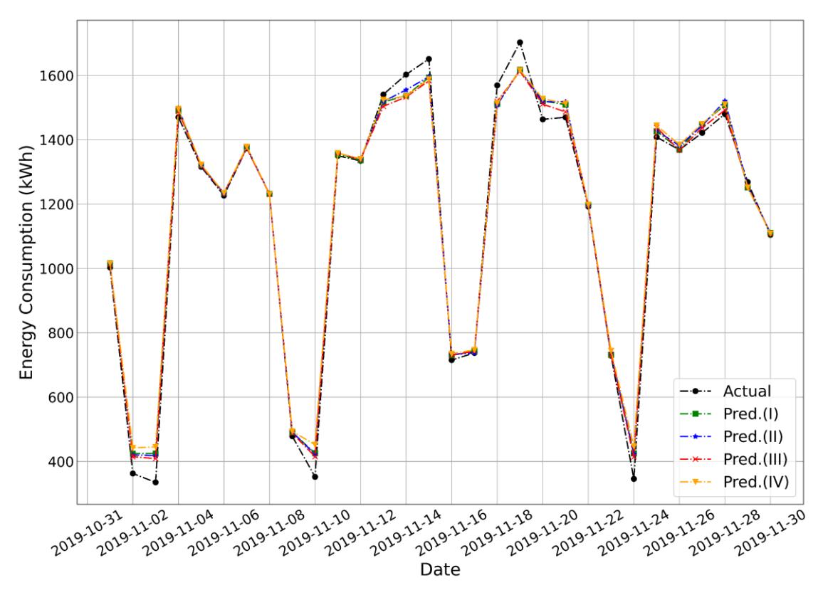
EL model deployment in the pre-pandemic period (November 2019).
Next, the models were deployed to predict building energy consumption during the pandemic from May to October 2020. Figure 7 shows a sample of the actual and predicted results. A decrease in the energy consumption was immediately apparent when comparing Figures 6 and 7. This trend was also observed in the boxplot in Figure 5. The statistical parameters presented in Table 5 confirm this, with a 55.48% reduction in mean energy consumption from the training data to the pandemic data. The reductions in the median further highlight a major shift in the central tendency. The pandemic data exhibited much lower variability, as shown by the standard deviations and IQR in Table 5. However, the pandemic data had numerous outliers above Q3, with the highest value reaching 1268.07 kWh. The observed changes were likely influenced by pandemic-related behavioral adaptations, such as reduced activity levels and remote working. These factors affect the prediction accuracy of models.
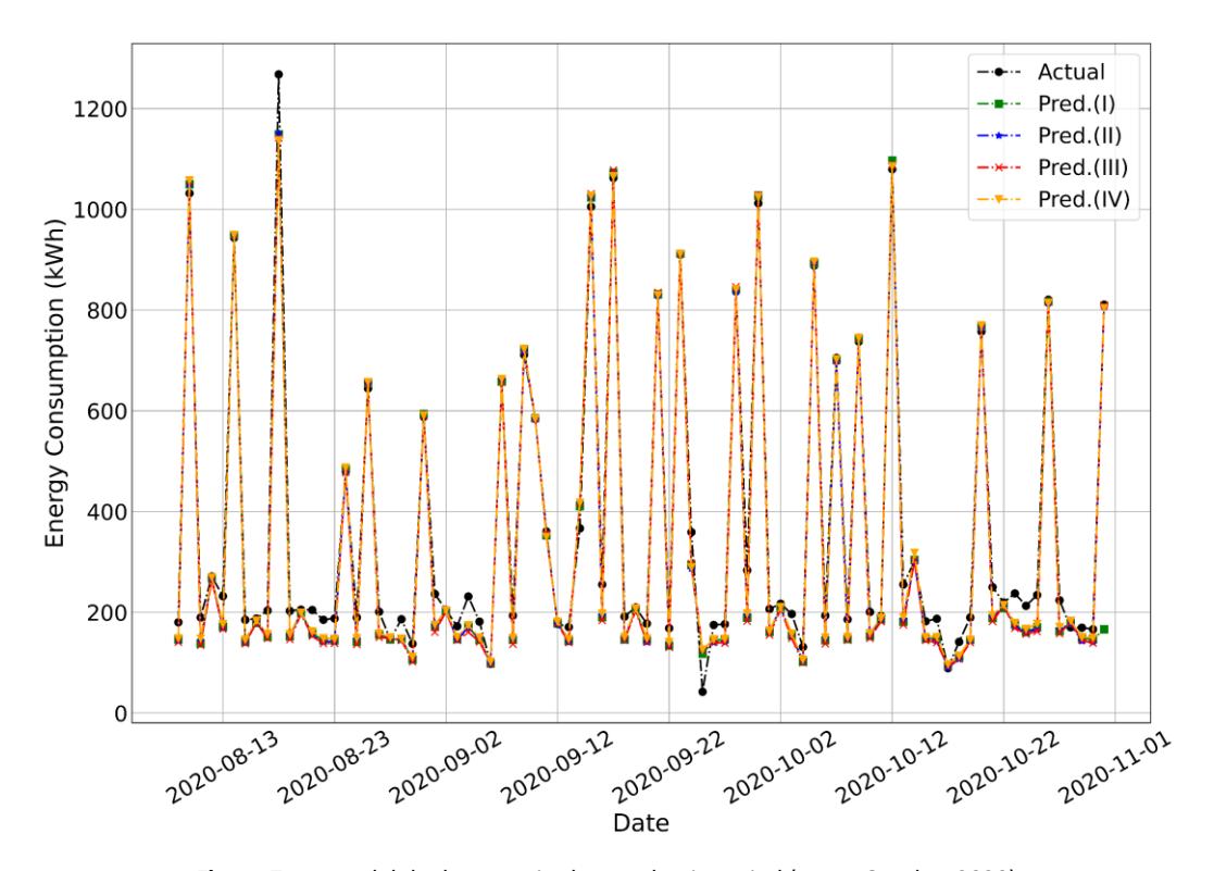
EL model deployment in the pandemic period (May - October 2020).
Table 7 summarizes the model performance in predicting the energy consumption data during the pandemic. In contrast with the previous results (Table 6), the best-performing model was Group I (MAPE 13.74%) instead of Group II (MAPE = 15.34%) with Group III (MAPE = 16.92%) still the least effective model. The results indicated that sliding windows are prominent features for energy consumption prediction. This finding demonstrates that the EL model trained with the sliding window feature possesses sufficient adaptability to disruptions in energy consumption patterns. Furthermore, this suggests that during the pandemic, building energy consumption was less correlated with the temperature. This is because buildings had few occupants due to social gathering restrictions during the pandemic. Occupancy levels are closely related to the utilization of HVAC systems in the building, which account for a significant portion of building energy usage (Asim et al., 2022).
| Alldays | Weekdays | Weekends | ||||||||
|---|---|---|---|---|---|---|---|---|---|---|
| Group | MAE | RMSE | MAPE | MAE | RMSE | MAPE | MAE | RMSE | MAPE | |
| (kWh) | (kWh) | (%) | (kWh) | (kWh) | (%) | (kWh) | (kWh) | (%) | ||
| I | 27.75 | 34.24 | 13.74 | 27.98 | 35.34 | 13.41 | 27.18 | 31.35 | 14.53 | |
| II | 49.45 | 36.86 | 15.34 | 30.24 | 38.40 | 14.72 | 31.66 | 36.27 | 16.89 | |
| III | 33.90 | 41.63 | 16.92 | 33.77 | 42.57 | 16.37 | 34.21 | 39.17 | 18.28 | |
| IV | 34.17 | 60.74 | 15.66 | 30.78 | 38.92 | 14.81 | 42.56 | 95.20 | 17.77 | |
Table 7 EL model deployment in the pandemic period (May - October 2020).
As in the case of the pre-pandemic data, the effect of weekends on the overall prediction error was analyzed. Based on Table 7, the differences in error metrics between weekdays and weekends were not greater than those during the prepandemic period (Table 6). This suggests that there was little difference in activity during weekdays and weekends, likely due to the COVID-19 restriction policies. However, the overall error metrics increased during this period compared with the pre-pandemic period. The increase in errors between testing during the pre-pandemic and pandemic periods aligns with the results observed in Arjomandi-Nezhad et al. (2022) and Wasesa et al. (2022). This phenomenon primarily resulted from drastic changes in electricity usage patterns during the pandemic. However, the model performed better (or at least had a comparable performance) than the models reported in Wasesa et al. (2022), where the MAPE ranged between 19.60 and 22.60%.
Conclusions
Energy consumption prediction has gained significant attention owing to its potential in BEMS development. Accurate prediction of building energy consumption is necessary to optimize resource allocation and promote sustainable energy usage. One of the main challenges in predicting building energy consumption is abrupt changes in building usage patterns. Extraordinary conditions such as the COVID-19 pandemic can significantly disrupt energy consumption patterns. Hence, this study aimed to develop an energy consumption model that can handle unexpected changes in energy consumption patterns. The combination of two basic learning methods (SVR and RF) in a two-layer stacking EL with temporal, sliding windows, temperature, and humidity input variables was demonstrated.
The EL model achieved a RMSE of 4.25–4.65 kWh, outperforming the SVR (67.92–87.88 kWh) and RF (38.76–50.62 kWh). The EL model was deployed during the pre-pandemic (November 2019) and pandemic (May– October 2020) periods. During the pre-pandemic period, the model provided accurate predictions despite the higher variability in November 2019 energy consumption, with a larger range and IQR compared to the training data. This shows that the sliding window features as input can effectively inform the model of changes in energy consumption patterns. Moreover, the deployment results during the pre-pandemic period suggest that temperature is a more prominent feature than humidity in improving prediction accuracy in this case. Adding humidity as a feature does not enhance the accuracy and can even degrade it. During the pandemic, the overall error metrics increased compared with the pre-pandemic period, with the best model MAPE values increasing from 3.77 to 13.74%. Despite this, the model outperformed similar studies and demonstrated adaptability to significant disruptions, including a 55.48% reduction in the mean energy consumption owing to COVID-19 restrictions. These results validate the effectiveness of the EL method combined with sliding windows and weather variables for energy consumption prediction.
This study contributes to the literature by proposing a model for building energy consumption during the COVID-19 pandemic, and comparing its performance during the pre-pandemic and pandemic periods. Most prior studies have focused on EL methods for specific applications, with limited attention paid to unexpected disruptions in energy consumption patterns during the COVID-19 pandemic. This study introduced a novel approach that combines a twolayer stacking ML model with sliding windows as features and weather variables during the COVID-19 pandemic. The novelty lies in exploring the use of sliding window features to enhance model adaptability and identify the weather variables that most significantly impact prediction performance.
This study had limitations that warrant further investigation. One limitation is the use of six months of training data (May – October 2019) and one month of test data (November 2019) for the pre-pandemic period. This limited timeframe may not have fully captured seasonal or cyclical trends (holidays or weather-related variations). Future research should focus on improving data availability so that extensive performance testing can be conducted. The methodology can also be enhanced by exploring other combinations of potential ML models in the EL framework using more diverse and extensive datasets. More accurate building energy consumption models can significantly contribute to BEMS improvements; however, a less complex model is also necessary for real-time applications.
Acknowledgements
This research was partially supported by an ITB Research Grant and a Research Grant of the Ministry of Research, Technology, and Higher Education.
Compliance with ethics guidelines
The authors declare that they have no conflict of interest or financial conflicts to disclose.
This article does not contain any studies with human or animal subjects performed by any of the authors.