
Introduction
Rapid development in Indonesia during this decade has led to the construction of numerous infrastructures on problematic soil, as exemplified by the Semarang–Demak toll road project. This toll road project is built on soft soil, which requires attention to issues regarding consolidation settlement. The pore water will be expelled from the soil during the consolidation process until the soil framework is capable of supporting the weight of the infrastructure above the soil (Hansbo, 1979). Consequently, soil improvement is necessary as a first step to support structures built on this soft soil. Preloading and Prefabricated Vertical Drain (PVD) are common methods used to improve soft soil conditions. The application of PVD is considered one of the most simple and efficient methods of ground enhancement for soft soils (Hansbo, 1981; Abuel-Naga, 2015; Zhafirah, 2021; Bergado et al., 2022). The principle behind these methods is to accelerate the consolidation settlement and increase strength (Spross & Larsson, 2021).
The settlement analysis and consolidation time observed in the field may differ from the predicted consolidation analysis estimated based on consolidation parameters obtained in the laboratory. This discrepancy can be attributed to various factors. The soil parameters used in the analysis can also significantly affect the settlement calculation results. Spross and Larsson (2021) noted that uncertainty in geotechnical parameters affects the prediction of the consolidation rate. The
consolidation rate refers to how quickly soil settles in response to loading. Furthermore, Muhammed et al. (2020) indicated that the settlement results would vary depending on the soil parameter data from tests conducted before or after construction.
The Terzaghi equation is an empirical method commonly used to calculate consolidation settlement. Several simplifying assumptions are present in the consolidation settlement analysis using Terzaghi's theory (Lekha et al., 2003). Consequently, the application of this theory to various practical problems can lead to significant errors (Abbasi et al., (2007); Raturi et al. (2023)). The calculation of consolidation settlement under Normally-Consolidated (NC) conditions using the Terzaghi one-dimensional method is influenced by the soil parameter, known as the compression index (Cc) (Das, 2010). Normally-Consolidated soil is characterized by a present effective overburden pressure that reflects the utmost pressure the soil has previously endured.
The compression index values can be determined through laboratory tests or empirical methods. Laboratory tests are conducted using an oedometer, and the Cc value is derived by plotting the slope of the relationship between the void ratio (e) and the logarithm of the applied stress (σ). Due to the low permeability of soft soils, consolidation testing often requires extended observation periods. Therefore, empirical methods are typically employed to obtain values for the soil compression index (Cc) based on the specific type of soil. For instance, Hough (1957) and Rendon-Herrero (1983), as cited in Das (2010), Skempton (1944) and Terzaghi and Peck (1967), as cited in Al-Khafaji & Andersland (1992) have provided several equations that describe the relationship between the soil compression index and initial void ratio (e0), specific gravity of the soil (Gs) and the Liquid Limit (LL). Additionally, the relationship between the soil compression index and the Liquid Limit can vary depending on the type of soil being analyzed (Al-Khafaji & Andersland, 1992).
The present study analyzes consolidation settlement resulting from compression caused by preloading and accelerated by Prefabricated Vertical Drains (PVD) in normally consolidated soft soil conditions. The analysis focuses on several stations (STA) along the Semarang-Demak toll road in Indonesia, specifically from STA 23+300 to STA 23+700, with various soil parameters. These stations were selected based on laboratory test undisturbed sample results and the availability of monitoring instrumentation data using Settlement Plate (SP). Consolidation analysis was conducted as a foundation for numerical analysis, which was subsequently validated against the final consolidation settlement results derived from field instrumentation observations. Parametric studies were employed to examine the consolidation parameters observed in the field, following the results of the Liquid Limit test. This study is particularly significant for road infrastructure in Indonesia, where site conditions are extensive and varied, presenting a range of soil parameters. Therefore, a comprehensive understanding of the soil parameters utilized in analyzing consolidation settlement is essential to designing soft soil infrastructure effectively in the future.
Methods
Material Parameters
This study takes an overview of the Semarang-Demak toll road, Indonesia, on the STA 23+300 to STA 23+700. The study area, shown in Figure 1, features numerous rice fields surrounding the STA location. Generally, the construction of this STA is situated on soft soil characterized by high water content, low permeability, and limited bearing capacity and shear strength. When subjected to construction loads, soil with these properties will undergo a consolidation process. The upper layer consists of soft clay (grey-brown) with a low Standard Penetration Test (SPT) value (N-SPT 3), indicating soft soil, as depicted in Figure 2. Thus, analyzing soil consolidation settlement is vital for infrastructure development on this soil type.
Figure 2 illustrates the soil stratification, with Figure 2(a) depicting the analysis from STA 23+050 to STA 23+400, and Figure 2(b) covering the analysis from STA 23+400 to STA 23+700. This stratification is based on Standard Penetration Test (SPT) data from STA 23+085, STA 23+185, and STA 23+650, and Cone Penetration Test (CPT) data from STA 23+250 and STA 23+450. The SPT testing adhered to SNI 4153:2008 standards, while the CPT testing followed SNI 2827:2008 guidelines. The soil stratification between STA 23+300 and STA 23+700 exhibits significant variation, ranging from soft clay to stiff clay, with several layers also identified as silty clay and sandy clay. Hard soil or soil exhibiting a high Standard Penetration Test (N-SPT of approximately 50) is typically found at a depth of around 50 meters and is characterized by very stiff clay. Additionally, the soil stratification from STA 23+450 to STA 23+700 was previously presented in a study by Sari et al. (2023). However, this study includes an updated elevation of the embankment height.
STA 23+300 to STA 23+700 as the location study (https://www.google.com/maps/, 2024).
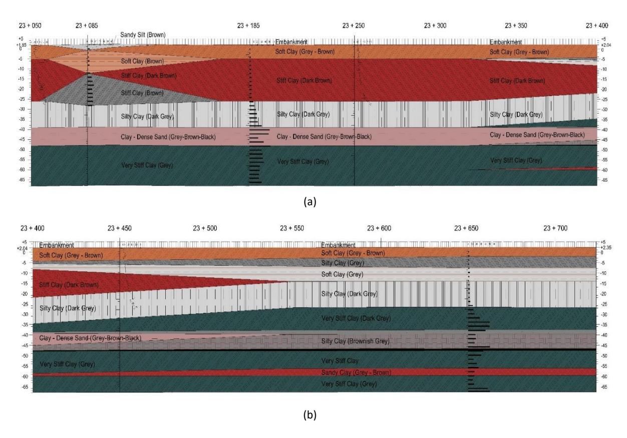
Soil stratification of the Semarang-Demak Toll Road from STA 23+050 to STA 23+400 (a) and from STA 23+400 to STA 23+700 (b).
Figure 3 illustrates the soil shear strength profile. The undrained shear strength values were derived from the relationship with the Standard Penetration Test (SPT) values based on Look (2007). As shown in Figure 3, the undrained shear strength values range from 20 kPa, particularly at depths between 5 and 10 meters. Soft soil is described as soil with an undrained shear strength ranging from 20 to 40 kPa, whereas very soft soil has an undrained shear strength of less than 20 kPa (Institution, 1986 in Elsawy et al., 2022). Therefore, the soil layers in the nine (9) Standard Test Areas (STAs) are classified as soft soil since the shear strength is less than 20 kPa. This classification is further supported by the results of the soil stratification analysis (Figure 2) conducted at STA 23+300 to STA 23+700, where the depth ranges approximately from 0 to 15 meters. The analysis reveals the presence of soft soil layers, which include the following soil types: Soft Clay (Grey - Brown), Silty Clay (Grey), and Soft Clay (Grey).
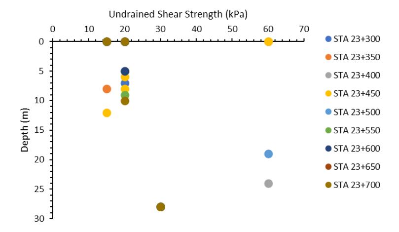
Figure 3 Undrained soil shear strength profile from STA 23+300 to STA 23+700.
Further, material parameters are essential for analyzing consolidation settlement. The material parameters were derived from the average soil characteristics at the nearest Station (STA). The initial assumptions were based on available laboratory test data: for STA 23+300 to STA 23+350, the parameters were based on laboratory testing conducted at STA 23+085, while for STA 23+400 to STA 23+700, the parameters were based on laboratory testing at STA 23+650. The laboratory results from STA 23+085 were considered primary data, whereas the results from STA 23+650 were classified as secondary data obtained from PT PP. These laboratory tests were performed on undisturbed samples collected from the Standard Penetration Test (SPT) at STA 23+085 and STA 23+650. Not all STAs were suitable for soil sampling due to location constraints. The soil settlement analysis was conducted to a depth of 30 meters, where the N-SPT value was approximately 10. As in Look (2007), soil with N-SPT 5-10 is categorized as firm or medium soft soil, which was used as a boundary in this study. Based on the stratification illustrated in Figure 2, the soil parameters were analyzed, which was subsequently used in numerical modeling.
In this study, the average values of soil parameters up to a depth of 30 meters were utilized to analyze the consolidation settlement of the soil. The calculation of soft soil consolidation settlement under Normally Consolidated (NC) conditions can be performed using the Terzaghi method. Empirical consolidation calculations employing this method require the input of soil parameters, specifically the Compression Index (C<sub>c</sub>) (Das, 2010). The values for the compression (C<sub>c</sub>) and recompression index (C<sub>r</sub>) in this study are illustrated in Figure 4. The C<sub>c</sub> and C<sub>r</sub> values presented in Figure 4 are averages from six soil samples taken at depths of 9.5-10 meters, 19.5-20 meters, 24.5-25 meters, and 29.5-30 meters. These values were determined from samples collected at STA 23+085 and STA 23+650 through laboratory testing (C<sub>c</sub>-lab and C<sub>r</sub>-lab) using an oedometer test (SNI 2812:2011). However, at depths of 4.5-5 meters and 14.5-15 meters, there were no available data for C<sub>c</sub> and C<sub>r</sub> values; therefore, these values were estimated using the empirical equations provided by Terzaghi and Peck (1967) (C<sub>c</sub>-empiric and C<sub>r</sub>-empiric), correlating them with the Liquid Limit (LL), as shown in Eq. (1). In Eq. (1), the LL value represents the Liquid Limit obtained from the Atterberg Limit test (SNI 1966:2008).
\[C_c = 0.009(LL - 10) \tag{1}\]
Figure 4 (a) shows that the \(C_r\) value for STA 23+300 to STA 23+350 is lower than the \(C_c\) value, consistent with Das (2010). However, Figure 4 (b) indicates that some \(C_r\) laboratory values exceed the \(C_c\) laboratory values at depths of 10 and 20 meters. This discrepancy introduces uncertainty in the laboratory results presented. Therefore, the \(C_c\) and \(C_r\) values used for analysis in this study were determined based on the correlation of soil stratification with existing literature (Look, 2007).
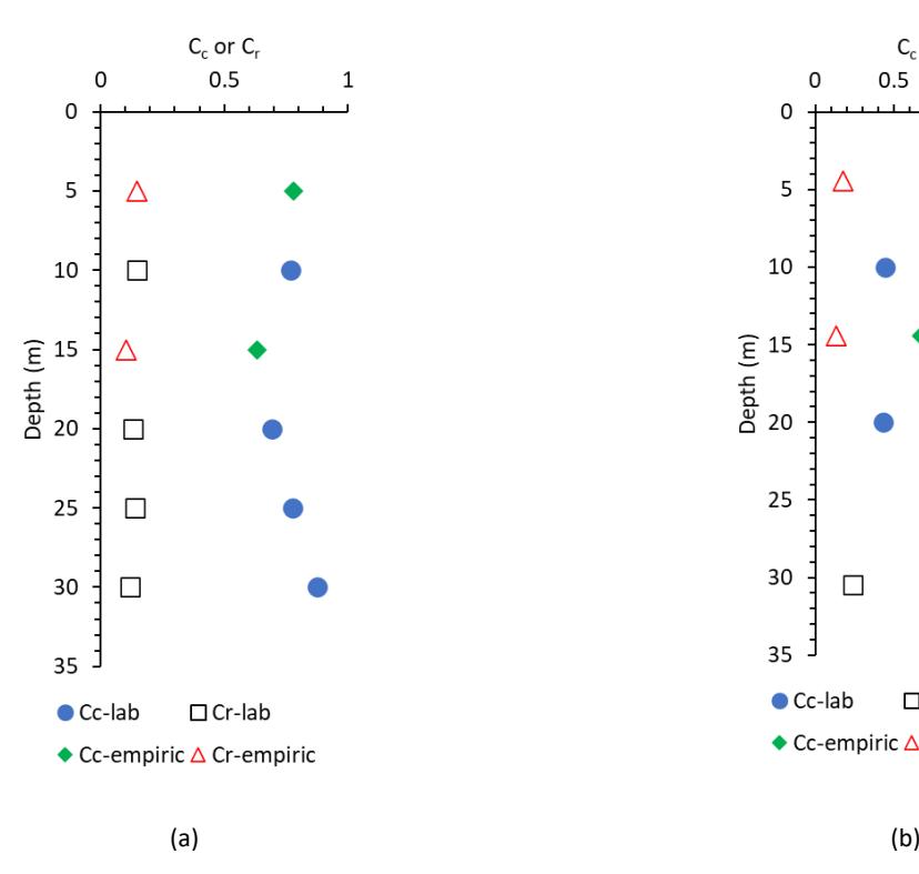
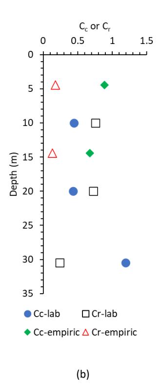
The availability of Cc and Cr values obtained from the consolidation test of soil samples at various locations: STA 23+300 to STA 300+350 (a); STA 23+400 to STA 23+700 (b).
Although soil stratification (as seen in Figure 2) reveals several layers of soil within the section from STA 23+300 to STA 23+700, this study focuses only on soft soil with a Standard Penetration Test (N-SPT) value of approximately 3. The SPT value of 2 - 5 is classified as soft soil (Look, 2007). Three (3) types of soil layers with an N-SPT value of approximately three were identified. The first layer is Soft Clay (Grey Brown), characterized by a coefficient of consolidation (Cc) of 0.886 and a coefficient of permeability (Cr) of 0.177. The second layer is Silty Clay (Grey), with a Cc value of 0.447 and a Cr value of 0.089. The third layer is Soft Clay (Grey), exhibiting a Cc value of 0.678 and a Cr value of 0.136. The thickness of each soil layer varies across different STAs, as illustrated in Figure 2 (soil stratification). Table 1 summarizes the soil layer thickness for each STA based on Figure 2.
Table 1 The thickness of each soil layer for each STA
| Layer of Soil | ||||
|---|---|---|---|---|
| STA | Layer | Depth (m) | Soil Type | |
| 23+300 | Layer 1 | 0 - 7 | Soft Clay (Grey Brown) | |
| Layer 1 | 0 - 6.5 | Soft Clay (Grey Brown) | ||
| 23+350 | Layer 2 | 6.5 - 6.7 | Silty Clay (Grey) | |
| Layer 3 | 6.7 - 8 | Soft Clay (Grey) | ||
| Layer 1 | 0 - 6.5 | Soft Clay (Grey Brown) | ||
| 23+400 | Layer 2 | 6.5 - 7.5 | Silty Clay (Grey) | |
| Layer 3 | 7.5 - 10.5 | Soft Clay (Grey) | ||
| Layer 1 | 0 - 6 | Soft Clay (Grey Brown) | ||
| 23+450 | Layer 2 | 6 - 8 | Silty Clay (Grey) | |
| Layer 3 | 8 - 12 | Soft Clay (Grey) | ||
| Layer 1 | 0 - 5.5 | Soft Clay (Grey Brown) | ||
| 23+500 | Layer 2 | 5.5 - 8.5 | Silty Clay (Grey) | |
| Layer 3 | 8.5 - 14.5 | Soft Clay (Grey) | ||
| Layer of Soil | ||||
|---|---|---|---|---|
| STA | Layer | Depth (m) | Soil Type | |
| Layer 1 | 0 - 5 | Soft Clay (Grey Brown) | ||
| 23+550 | Layer 2 | 5 - 9 | Silty Clay (Grey) | |
| Layer 3 | 9 - 16,5 | Soft Clay (Grey) | ||
| Layer 1 | 0 - 5 | Soft Clay (Grey Brown) | ||
| 23+600 | Layer 2 | 5 - 9.5 | Silty Clay (Grey) | |
| Layer 3 | 9.5 - 16.5 | Soft Clay (Grey) | ||
| Layer 1 | 0 - 4.5 | Soft Clay (Grey Brown) | ||
| 23+650 | Layer 2 | 4.5 - 10 | Silty Clay (Grey) | |
| Layer 3 | 10 - 16.5 | Soft Clay (Grey) | ||
| Layer 1 | 0 - 4.5 | Soft Clay (Grey Brown) | ||
| 23+700 | Layer 2 | 4.5 - 10 | Silty Clay (Grey) | |
| Layer 3 | 10 - 16.5 | Soft Clay (Grey) | ||
In numerical modeling, in addition to soil consolidation parameter values, other soil parameter values are also required, as presented in Table 2. Table 2 provides the soil parameters for the original soil (subgrade) and the embankment (preloading). In this study, only the unit weight value was obtained from laboratory test results for the embankment parameters. In contrast, the other parameter values were derived based on correlations between literature studies (Look, 2007) and soil types. For the subgrade, the unit weight (\(\gamma\)), void ratio (e), and Over-Consolidated Ratio (OCR) were determined through laboratory tests. At the same time, the Pre-overburden Pressure (POP) parameters were calculated based on the relationship between unit weight and soil depth. Meanwhile, additional soil parameters, including soil stiffness (elastic modulus (E) and Poisson's ratio (v)), permeability (k), and soil strength (cohesion (c) and friction angle (\(\phi\))), were obtained using correlations from literature studies (Look, 2007) and soil types, as illustrated in Figure 2.
The permeability coefficient consists of horizontal and vertical permeability. Horizontal permeability refers to a soil's ability to transmit fluid in a direction perpendicular to gravity, while vertical permeability describes the ability to transmit fluid along the direction of gravity. The horizontal and vertical permeability coefficient must be adjusted to the initial permeability coefficient values due to the installation of Prefabricated Vertical Drains (PVD), which can alter the permeability coefficient. This adjusted permeability coefficient is referred to as the equivalent permeability coefficient. Saputro et al. (2018) suggested that soil permeability (k) used in the numerical study was about one-half of the k value determined from the laboratory test. In this study, the vertical equivalent permeability value was calculated using the method proposed by Chai et al. (2001), and the horizontal equivalent permeability value was determined based on the approach by Hird et al. (1992), as shown in Eqs. (2) and (3).
\[k_{ve} = \left(1 + \frac{2.5I^2}{\mu D_e^2} \frac{k_h}{k_v}\right) k_v \tag{2}\]
\[\frac{k_{np}}{k_n} = \frac{0.67}{\ln(n) - 0.75} \tag{3}\] where \(k_{ve}\) is the vertical equivalent permeability; \(k_{hp}\) is the horizontal equivalent permeability non-smear zone condition; \(k_v\) is the initial vertical permeability coefficient; \(k_h\) is the initial horizontal permeability coefficient; l is the length of PVD (\(H_{dr}\)); \(\mu\) is the correction factor; \(D_e\) is the PVD range diameter; n is the \(D_e/d_w\) (\(d_w\) is the diameter of drain).
| Soil Parameters | Unit | Embankment | Original Soil (Subgrade) | ||
|---|---|---|---|---|---|
| 3011 Parameters | Unit | Empankment | Layer 1 | Layer 2 | Layer 3 |
| Elastic Modulus (E) | kN/m² | 20000 | 2000 | 2000 | 5000 |
| Poisson's Ratio (\(\nu\)) | 0.3 | 0.45 | 0.45 | 0.45 | |
| Unit Weight ( \(\gamma\)) | kN/m³ | 15.6 | 15.75 | 15.98 | 15.82 |
| Saturated Unit Weight (\(\gamma_{sat}\)) | kN/m³ | 17.6 | 15.605 | 15.732 | 15.559 |
| Initial Void Ratio (\(e_o\)) | 0.5 | 1.719 | 1.616 | 1.737 | |
| Permeability coeff. \((k_x)\) | m/day | 1.728 | 0.00030181 | 0.00030181 | 0.00030181 |
| Permeability coeff. \((k_y)\) | m/day | 0.864 | Depending on the layer thickness | nickness | |
| Permeability coeff. \((k_z)\) | m/day | 1.728 | 0.00030181 | 0.00030181 | 0.00030181 |
| Over Consolidation Ratio ( | OCR) | - | 1 | 1 | 1 |
| Pre-overburden Pressure (POP) kN/m2 | - | Depending on the unit weight and layer thickness | d layer thickness | ||
| Cohesion (c) | kN/m² | 19 | 20 | 20 | 15 |
| Frictional Angle (φ) | 0 | 25 | 15 | 15 | 15 |
Table 2 The input parameter for numerical modelling.
Numerical Modeling
This study utilized numerical modeling to analyze consolidation settlement and identify the consolidation parameters that influence the final consolidation settlement result. The modeling analysis is complex in achieving results accurately reflecting actual field conditions. The model must be designed to replicate these conditions closely. This modeling approach has been extensively studied, as the results are significantly affected by determining material model parameters and selecting soil materials (Le et al., 2018).
Numerical analysis in this study was conducted using MIDAS GTS NX 2021 (V.1.1). MIDAS GTS NX is a specialized program developed for addressing geotechnical problems (Cao & Hang, 2021). The material model applied was the Mohr-
Coulomb (MC) model for embankment soil and the Modified Cam-Clay Model (MCC) for the original soil/subgrade. The geometric modeling of the toll road cross-section is illustrated in Figure 5. In contrast, the modeling of Prefabricated Vertical Drains (PVD) and the toll road cross-section in MIDAS is shown in Figure 6.
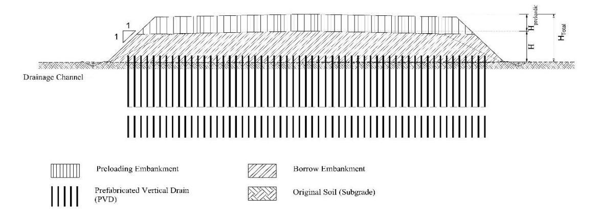
Figure 5 Typical cross-section and preloading design.
Based on Figure 5, this study utilized a triangular-type PVD with a depth of 22 meters, a width of 100 mm, a thickness of 3 mm, and a spacing of 0.9 meters. The sketch of the triangular-type PVD, complete with its width and thickness, is typical of previous studies (Sari et al., 2023). The preloading fill (embankment) is positioned above the subgrade with a slope ratio of 1:1. The total height of the embankment (\(H_{total}\)) consists of the borrow embankment height (H) and the preloading height (\(H_{preloading}\)). This configuration ensures that, after consolidation settlement occurs, the embankment height remains consistent with the planned highway elevation. Additionally, a drainage channel is provided to facilitate the removal of excess pore water.
Furthermore, the STA sections reviewed in this study feature different preloading stages, as shown in Table 3. These preloading stages vary between 6 and 8 stages. The lowest preloading height was 4.70 meters at STA 23+400, while the highest was 5.69 meters at STA 23+700. The total time required to complete the preloading of this embankment was 323 days based on Settlement Plate observation. Each embankment stage comprises two components: embankment time and leaving time. The embankment time, also called construction time, is the duration required to construct the embankment. On the other hand, the leaving time stage represents the waiting period before the next embankment stage begins. During this phase, time is allocated for consolidation to occur, allowing excess pore pressure to dissipate. This study also interprets leaving time as the consolidation time between each embankment stage. The determination of preloading stages and their durations was based on field observations using Settlement Plate instrumentation. Consequently, the geometric model of each STA varies according to the respective preloading height. The meshing used in this modeling is quadrilateral in type, with a size of 1 × 1 m². Reducing the mesh size results in finer meshing for more detailed modeling.
| STA | Embankment Stages | Preloading Height (m) | STA | Embankment Stages | Preloading Height (m) |
|---|---|---|---|---|---|
| 23+300 | 7 | 5.02 | 23+550 | 6 | 5.19 |
| 23+350 | 7 | 5.29 | 23+600 | 8 | 5.52 |
| 23+400 | 6 | 4.70 | 23+650 | 8 | 5.37 |
| 23+450 | 6 | 5.25 | 23+700 | 7 | 5.69 |
| 23+500 | 6 | 5.22 |
Table 3 Stages of embankment from STA 23+300 to STA 23+700.
In modeling using Midas GTS NX, as shown in Figure 6, the soil layer was divided into two conditions. The first was the original soil layer or subgrade, which was in a consolidated condition, and the second was the preloading embankment layer in an unconsolidated condition. This subgrade layer consists of approximately five layers with different soil types under the preloading (to a depth of 30 m). This variation of soil layers was based on soil stratification (Figure 2). In addition, to match the actual conditions, the original upper and lower layers and the geometry of the PVD model were also created in a drained condition. The model is illustrated clearly in Figure 6. The figure shows an example of a geometry model on STA 23+600, which is typical of the other station geometry model. Hence, the distinctions between
each STA were the height of the preloading embankment (Table 3) and the depth of the soil stratum, which is determined by its stratification pattern (Figure 2).
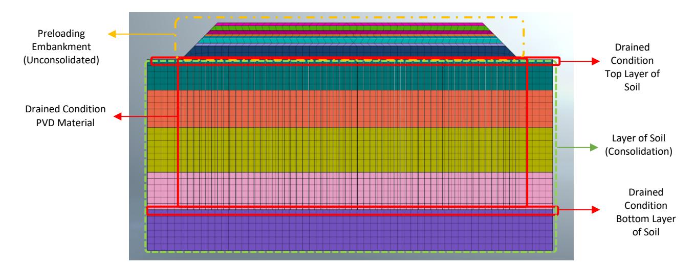
Figure 6 Midas GTS NX Model Geometry at STA 23+600.
Furthermore, modeling can be conducted by setting construction stages, including the initial stage, the first embankment through to the last embankment, and the leaving time period. The leaving time varied for each STA, depending on the embankment stage being executed. As previously explained, each stage had a different duration, determined based on observations from Settlement Plate instrumentation in the field. As a result, the modeling outcomes provided the final consolidation settlement as well as a relationship between settlement and time, as to the observations made using settlement plates in the field.
Modeling results may differ from actual field results. Unreliable predictions can be attributed to various factors, including soil evaluation (Hiep & Chung, 2018). Therefore, the back analysis method can be employed to refine material parameters that influence consolidation settlement. This method is widely applied in the geotechnical field to determine material parameters (Fakhimi et al. (2004); Lam et al. (2015); Hiep & Chung (2018)). Unlike the Terzaghi equation, the consolidation settlement value in MIDAS numerical modeling is influenced by the Slope of the Consol Line (\(\lambda\)) and the Slope of the Over Consol Line (\(\lambda\)) (MIDAS GTS NX, 2023). These two factors depend on soil consolidation parameters such as the compression index (\(\lambda\)) and the recompression index (\(\lambda\)). By evaluating these parameters, the final consolidation settlement values can be approximated to align with actual soil consolidation parameters in the field. This ensures that the modeled settlement corresponds to the observation period in the field and matches the magnitude of the final consolidation settlement. Eqs. (4) and (5) represent the calculations for the Slope of the Consol Line and the Slope of the Over Consol Line, respectively (Midas GTS NX, 2023).
\[\lambda = \frac{C_c}{2.303} \tag{4}\]
\[k = \frac{C_r}{2.303} \tag{5}\]
This study applied the back analysis method to evaluate consolidation parameters, compression index (C<sub>c</sub>), and the recompression index (C'). This approach involved comparing the final consolidation settlement results from the numerical analysis with the actual settlement observed in the field. Previous research has emphasized that numerical analysis results must be assessed against actual field observations (Syahbana & Sarah, 2013). Based on this principle, the modeling results in this study were verified using the settlement plate instrumentation data collected from the field observation.
Results
The consolidation settlement analysis for each STA conducted in this study was based on the existing embankment stages, which have varying preloading heights, as shown in Table 3. Figure 7 presents a typical relationship between the preloading embankment stages and the settlement observations obtained using Settlement Plate instrumentation for
STA 23+600. As illustrated in Figure 7, there are eight embankment stages. The total observation period using the Settlement Plate for all embankment stages was 323 days. The final observation was made on July 29, 2022, with a preloading embankment height of 5.52 meters (Table 3) and a final consolidation settlement of 1580 mm (1.58 m) based on the settlement plate instrumentation observation. Variations in embankment stages influenced the settlement graph observed through the Settlement Plate instrumentation.
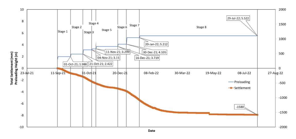
Graph of preloading embankment height and settlement observation using Settlement Plate on STA 23+600.
The final consolidation settlement analysis was conducted using MIDAS GTS NX modeling, as shown in Figure 8. The fundamental concept of applying the finite element method in numerical modeling is to find practical solutions for complex field problems (Rao, 2005, as cited in Wong & Somanathan, 2019). In this study, the settlement analysis focused on the final settlement or 100% degree of consolidation. Verification was performed by comparing the final consolidation settlement results with field instrumentation data from the Settlement Plate observation, where the settlement considered was the value observed at the end of the preloading period. For instance, at STA 23+600, the settlement at the end of the observation period was 1.58 meters (Figure 7).
Figure 8 indicates a significant difference between the numerical modeling results and the actual final consolidation settlement observed in the field. The results of this analysis are based on the input parameters in Table 2. The numerical modeling results were lower than the field settlements, which aligns with the findings of Islam et al. (2012), who studied settlementsin embankments. According to Islam et al. (2012), the settlement analysis with Modified Cam Clay predicted using finite element modeling analysis was lower than expected when compared to field settlement measurements. Moreover, in this study, based on Figure 8, the largest deviation occurred at STA 23+550, where the numerical modeling result (1.26 meters) was 19.77% lower than the settlement plate observation result (1.57 meters). Conversely, the lowest deviation was recorded at STA 23+350, with a difference of 9.12% between the numerical modeling result (1.37 meters) and the Settlement Plate observation result (1.51 meters).
In their study, Muhammed et al. (2020) stated that the initial model provided a pattern that did not match with field conditions, necessitating modifications and back-analysis calculations, referred to as Class C predictions. Class C predictions are estimations made after modifying the soil layers and adjusting influencing parameters to improve prediction accuracy. Hence, this study conducted a back-analysis method to obtain new consolidation parameter values, ensuring that the final consolidation settlement results closely matched field observations. The result aligns with the findings of Le et al. (2018), which highlight that numerical models, especially those using the Modified Cam-Clay model, can effectively predict embankment behavior but require adjustments to soil parameter selection.
In this numerical modeling, the first analysis involved varying the Cc value while keeping the Cr value constant. Subsequently, the Cr value was altered while maintaining a constant Cc value. The parameter adjustments were performed to achieve final consolidation settlement results that closely aligned with field data obtained through settlement plate instrumentation. The concept behind this parameter adjustment was based on a linear regression approach, which employs dependent and independent variables (Schober et al., 2018).
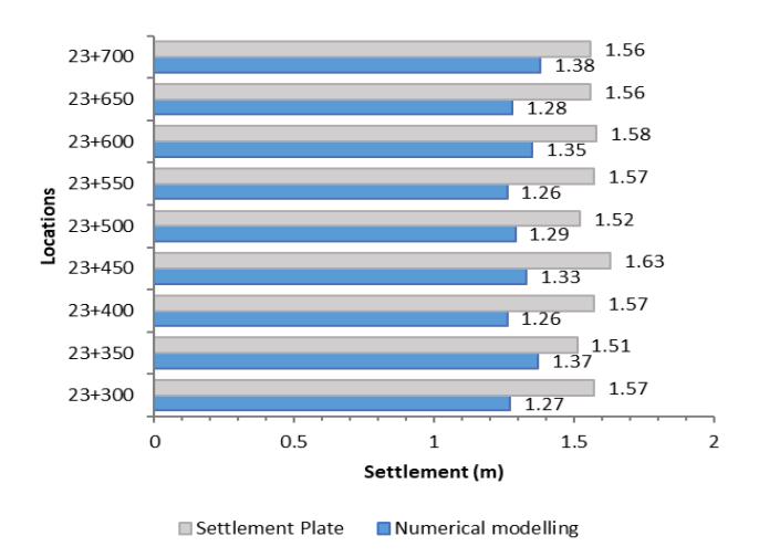
Comparison of the final settlement at initial simulation using input parameter in Table 2.
The consolidation settlement process occurs in the top three soft soil layers as established in the earlier section entitled 'Methods'. The Cc and Cr values analysis was initially conducted on the first layer, which consists of soft clay soil (greybrown). This layer was selected for initial optimization because it is the softest among the three layers, which is indicated by the SPT value in the soil stratification profile in Figure 2. Focusing on the softest layer allows for an accurate analysis of how changes in consolidation parameters affect consolidation settlement. Table 4 provides an example of the corrected Cc values, while Table 5 summarizes the Cr value adjustments for STA 23+600.
Table 4 Determination of compression index (Cc) values in STA 23+600 for numerical analysis evaluation.
| STA | Trial | Compression Index (Cc) | Recompression Index (Cr) | Final Settlement (Sc)(m) | Settlement Plate Result (m) |
|---|---|---|---|---|---|
| 1 | 0.712 | 0.177 | 1.123 | ||
| 2 | 0.798 | 0.177 | 1.233 | ||
| 23+600 | 3 | 0.886 | 0.177 | 1.350 | 1.582 |
| 4 | 0.992 | 0.177 | 1.486 | ||
| 5 | 1.078 | 0.177 | 1.601 |
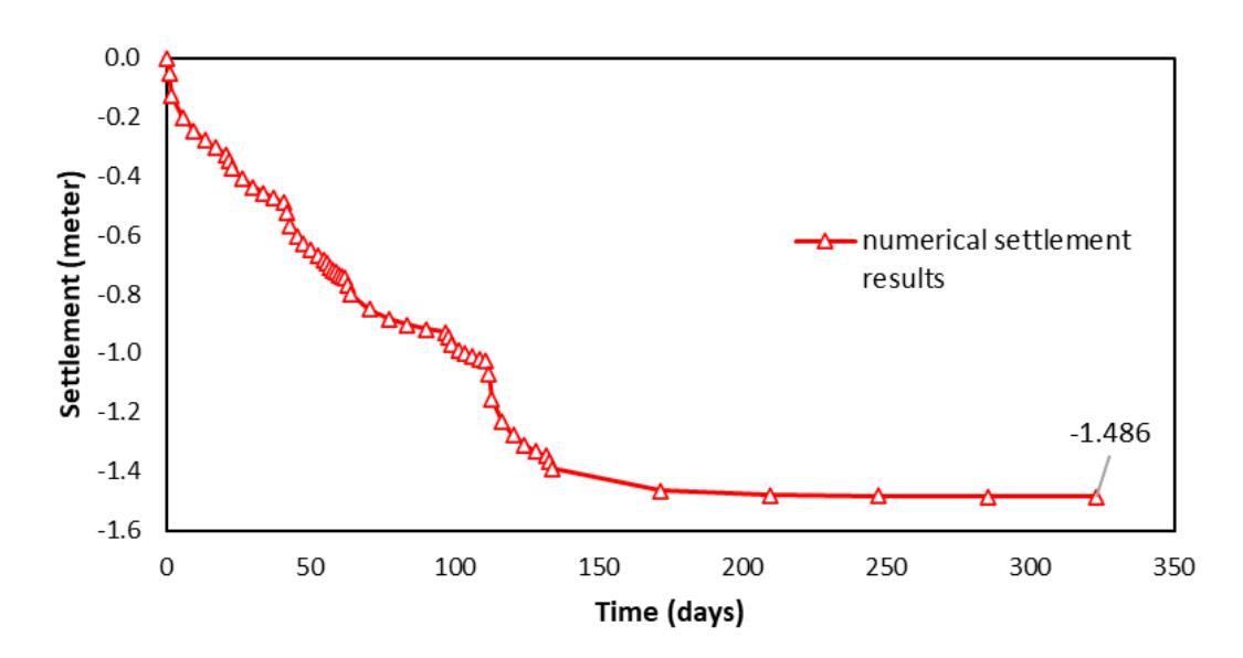
Numerical analysis of consolidation settlement using Midas at STA 23+600 (trial 4 from Table 4; Cc = 0.992; Cr = 0.177).
1.582
23+600
In the first layer of STA 23+600, the initial values of Cc and Cr were 0.886 and 0.177, respectively. These initial values produced a settlement of 1.350 m (can be seen in Figure 8 or Table 4 in the third trial). Subsequent modifications involved varying the Cc value (independent variable) while keeping the Cr value constant (dependent variable), as shown in Table 4. Based on the evaluation, the optimum Cc value was determined to be 0.992, resulting in a final settlement of 1.486 m at 323 days, closely approximating the Settlement Plate observation result of 1.582 meters (Table 4). The final settlement here refers to the consolidation settlement at the end of the consolidation process, which was conducted using a combination of the PVD and preloading methods. Figure 9 illustrates an example of a consolidation settlement graph, showing a final settlement of 1.486 meters achieved at the end of the 323-day consolidation period.
Moreover, with a constant Cc value of 0.992, the Cr value was varied, and the optimal Cr value was found to be 0.223, resulting in a settlement value of 1.513 meters (Table 5). This final settlement is close to the Settlement Plate value of 1.582 meters. The optimization steps for Cc and Cr were also carried out progressively on layers 2 and 3 at STA 23+600. As a result, the final numerical settlement value was found to be 1.579 m, with a deviation of 0.191% from the settlement plate (as seen in Table 7). The process of determining the Cc and Cr values was repeated for all STAs reviewed.
| STA | Trial | Compression Index (Cc) | Recompression Index (Cr) | Final Settlement (Sc)(m) | Settlement Plate Result (m) |
|---|---|---|---|---|---|
1 0.992 0.152 1.470
0.992 0.223 1.513 0.992 0.398 1.617 0.992 0.421 1.630 0.992 0.513 1.682
Table 5 Determination of recompression index (Cr) values at STA 23+600 for numerical analysis evaluation.
| Table 6 | Correction of consolidation parameters (numerical). |
|---|
| Layer of Soil Correction Parameter | Correction Factor | ||||||
|---|---|---|---|---|---|---|---|
| STA | Layer | Depth (m) | Soil Type | Cc | Cr | Cc | Cr |
| 23+300 | Layer 1 | 0 - 7 | Soft Clay (Grey Brown) | 0.920 | 0.465 | 1.0 | 2.6 |
| Layer 1 | 0 - 6.5 | Soft Clay (Grey Brown) | 0.931 | 0.239 | 1.1 | 1.4 | |
| 23+350 | Layer 2 | 6.5 - 6.7 | Silty Clay (Grey) | 0.532 | 0.181 | 1.2 | 2.0 |
| Layer 3 | 6.7 - 8 | Soft Clay (Grey) | 0.763 | 0.228 | 1.1 | 1.7 | |
| Layer 1 | 0 - 6.5 | Soft Clay (Grey Brown) | 1.016 | 0.275 | 1.1 | 1.6 | |
| 23+400 | Layer 2 | 6.5 - 7.5 | Silty Clay (Grey) | 0.617 | 0.217 | 1.4 | 2.4 |
| Layer 3 | 7.5 - 10.5 | Soft Clay (Grey) | 0.848 | 0.264 | 1.3 | 1.9 | |
| Layer 1 | 0 - 6 | Soft Clay (Grey Brown) | 0.971 | 0.316 | 1.1 | 1.8 | |
| 23+450 | Layer 2 | 6 - 8 | Silty Clay (Grey) | 0.532 | 0.228 | 1.2 | 2.6 |
| Layer 3 | 8 - 12 | Soft Clay (Grey) | 0.763 | 0.275 | 1.1 | 2.0 | |
| Layer 1 | 0 - 5.5 | Soft Clay (Grey Brown) | 0.980 | 0.245 | 1.1 | 1.4 | |
| 23+500 | Layer 2 | 5.5 - 8.5 | Silty Clay (Grey) | 0.540 | 0.157 | 1.2 | 1.8 |
| Layer 3 | 8.5 - 14.5 | Soft Clay (Grey) | 0.771 | 0.204 | 1.1 | 1.5 | |
| Layer 1 | 0 - 5 | Soft Clay (Grey Brown) | 1.006 | 0.269 | 1.1 | 1.5 | |
| 23+550 | Layer 2 | 5 - 9 | Silty Clay (Grey) | 0.567 | 0.181 | 1.3 | 2.0 |
| Layer 3 | 9 - 16,5 | Soft Clay (Grey) | 0.798 | 0.228 | 1.2 | 1.7 | |
| Layer 1 | 0 - 5 | Soft Clay (Grey Brown) | 0.992 | 0.223 | 1.1 | 1.3 | |
| 23+600 | Layer 2 | 5 - 9.5 | Silty Clay (Grey) | 0.553 | 0.135 | 1.2 | 1.5 |
| Layer 3 | 9.5 - 16.5 | Soft Clay (Grey) | 0.784 | 0.182 | 1.2 | 1.3 | |
| Layer 1 | 0 - 4.5 | Soft Clay (Grey Brown) | 1.006 | 0.240 | 1.1 | 1.4 | |
| 23+650 | Layer 2 | 4.5 - 10 | Silty Clay (Grey) | 0.567 | 0.152 | 1.3 | 1.7 |
| Layer 3 | 10 - 16.5 | Soft Clay (Grey) | 0.798 | 0.199 | 1.2 | 1.5 | |
| Layer 1 | 0 - 4.5 | Soft Clay (Grey Brown) | 0.970 | 0.207 | 1.1 | 1.2 | |
| 23+700 | Layer 2 | 4.5 - 10 | Silty Clay (Grey) | 0.530 | 0.119 | 1.2 | 1.3 |
| Layer 3 | 10 - 16.5 | Soft Clay (Grey) | 0.762 | 0.166 | 1.1 | 1.2 | |
Table 6 summarizes the corrected consolidation parameters (Cc and Cr) used to obtain the final consolidation settlement correction for each layer of soil. At STA 23+300 there is only one layer of soil in the form of soft clay (grey-brown). This is because, based on the stratification profile (Figure 2), the layer after the soft soil is stiff clay (dark brown), which is not considered in the consolidation settlement analysis. The correction factor in Table 6 is derived by comparing the corrected consolidation parameters (obtained from numerical analysis) with the laboratory consolidation parameters (initial values). Then, the final consolidation settlement results are in accordance with observations of settlement in the field with settlement plate instrumentation after the correction factors are applied. The average correction factor for Cc in soft clay (grey-brown), silty clay (grey-brown), and soft clay (grey) soils are 1.1, 1.2, and 1.2, while the average correction factor for Cr is 1.6, 1.9, and 1.6.
Further, Table 6 shows that the compression index (Cc) correction in the Soft Clay (Grey Brown) soil type is approximately 0.98, for the Silty Clay (Grey) soil type it is around 0.55, and for the Soft Clay (Grey) soil type it is approximately 0.79. Therefore, the softer the soil, the higher the compression index value. The compression indices, from smallest to largest, are in the following order: Silty Clay (Grey), Soft Clay (Grey), and Soft Clay (Grey-Brown), as shown in Figure 10(a). Silty Clay, or clayey silt soil, has a higher SPT value than Soft Clay or soft clay soil.
Meanwhile, for the recompression index (Cr) correction, the Soft Clay (Grey-Brown) soil type has a value of around 0.28, the Silty Clay (Grey) soil type has a value of about 0.17, and the Soft Clay (Grey) soil type has a value of approximately 0.22. Similar to the compression index, the softer the soil, the higher the recompression index value, as shown in Figure 10 (b).
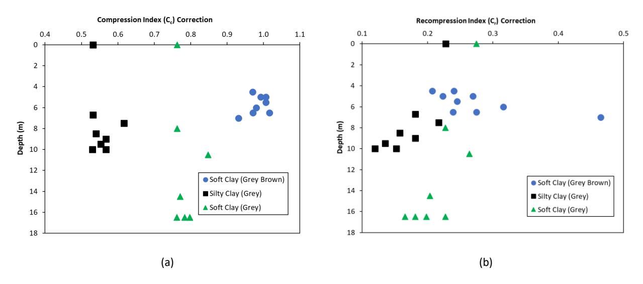
Correction consolidation parameter values based on soil type and depth: compression index (Cc) (a) and recompression index (Cr) (b).
The results of this study are also supported by Liao & Zhao (2020), which examined the physical characteristics of cohesive soil. Their empirical calculations of the compression index based on water content show that the softer the clay, the higher the compression index. These findings are consistent with the results of laboratory tests. In Liao & Zhao's study, the smallest to largest compression indexes were observed in the following order: hard clay, firm clay, and soft clay soil types. Similarly, Ayeldeen et al. (2021) analyzed the value of the soil compression index based on the soil Liquid Limit (LL). According to their soil test data, the Cc value at depths of up to about 15 meters for soft silty sand to silty clay soil (defined as Clay 1) types is lower than the Cc value of soft clay soil (defined as Clay 2) at depths above 15 meters. This suggests that soft clay soil types have a higher Cc value than hard clay.
A recapitulation of the deviations in the results of the final consolidation settlement correction can be seen in Table 7. The results of the numerical analysis of the final consolidation settlement are compared to the settlement plate observations, which show a deviation of less than 1%. The largest deviation is found at STA 23+550, with a deviation of 0.282%, while the smallest is at STA 23+700, with a deviation of 0.075%. These numerical settlement results (final consolidation settlement correction) differ from those of the previous numerical settlement analysis (Figure 8) due to changes in the consolidation parameters;specifically, the compression index (Cc) and recompression index (Cr), obtained through back analysis on Midas.
Discussion
Table 7 shows that with the alteration of Cc and Cr values, the difference in the final consolidation settlement result from numerical analysis compared to the Settlement Plate observation becomes smaller, with a deviation below 1%. Therefore, the compression index (Cc) value is crucial in geotechnical design (Díaz & Spagnoli, 2024). The difference between the new parameter values, the compression index (Cc) and the recompression index (Cr), and the initial Cc and Cr values varies significantly depending on the optimum final consolidation settlement analysis conducted during evaluation using the back analysis method. However, this can also be influenced by the height of the preloading embankment. The height of the preloading embankment can affect the height of the embankment after settlement. The higher the height of the preloading embankment, the greater the final embankment height (Fatmawati et al., 2023). Meanwhile, in the research of Fatmawati et al. (2023), which was conducted at four different STAs, the settlement that occurred was not in line with the increase in the height of the embankment. Alibeikloo et al. (2020) stated that the preloading duration was a more compelling factor than the preloading height. Consequently, the changes in these consolidation parameters make it quite challenging to categorize and analyze their behavioral patterns.
| Final Consolidation Settlement (m) | |||
|---|---|---|---|
| STA | Numerical Modeling | Settlement Plate | Deviation (%) |
| 23+300 | 1.570 | 1.573 | 0.221 |
| 23+350 | 1.499 | 1.509 | 0.639 |
| 23+400 | 1.565 | 1.574 | 0.563 |
| 23+450 | 1.633 | 1.634 | 0.064 |
| 23+500 | 1.519 | 1.520 | 0.061 |
| 23+550 | 1.561 | 1.565 | 0.282 |
| 23+600 | 1.579 | 1.582 | 0.191 |
| 23+650 | 1.556 | 1.559 | 0.217 |
| 23+700 | 1.560 | 1.561 | 0.075 |
Table 7 Comparison of final consolidation settlement using back analysis method.
Soil consolidation settlement is a time-dependent phenomenon influenced by the permeability coefficient of the existing soft soil. Additionally, changes in permeability have similarities to changes in compressibility (Lekha, et al., 2003). Figure 11 shows a comparison of the settlement curve over time between numerical modeling (with initial Cc and Cr; and corrected Cc and Cr (modified)) and the results of Settlement Plate (SP) observations for all of the STAs reviewed in this study. This corrected Cc and Cr is based on optimizations done previously. It can be seen in Figure 11, with changes in the Cc and Cr values, the settlement curve over time for the numerical analysis closely approximates the settlement observed with the settlement plate. The settlement time used was 323 days for each stage, as observed during the preloading stages and Settlement Plate observations in the field. However, the time for each embankment stage varies across different STAs. Figure 11 also highlights how different analysis models can influence the settlement patterns that develop over time.
Figure 11 (a) presents the settlement profile with Cc and Cr corrections based on the average parameters of the top three (3) soft soil layers at each STA. In this condition, sample analysis was conducted on STA 23+300, and STA 23+600 to STA 23+700. The analysis in Figure 11 (a) does not take into account the equivalent horizontal and vertical permeability coefficients, nor does it include the leaving time condition for each embankment stage. Meanwhile, Figures 11 (b) and 11 (c) present the settlement profiles before and after the correction of the Cc and Cr values for nine (9) STAs on the top three (3) soft soil layers reviewed (as explained in the 'Methods' and study boundary), from STA 23+300 to STA 23+700. The analysis of the Cc and Cr parameters in the top three (3) soft soil layers was carried out in stages, as explained in the 'Results' section. The analysis in Figure 11 (b) and Figure 11 (c) was carried out by considering the equivalent horizontal and vertical permeability coefficients. Unlike the condition in Figure 11 (a), in the Figure 11 (b) and Figure 11 (c) provide the leaving time stages for each embankment stage.
The results of the settlement plotting show that the analysis is more accurate when performed on each soil layer (Figures 11(b) and 11(c)) compared to averaging the overall parameter values of the soil (Figure 11(a)). In Figure 11(a), although the final value of the consolidation settlement is the same as the Settlement Plate (with a deviation of 5%), the consolidation settlement curve is still sloping. This suggests that the consolidation settlement has not yet been completed. The numerical results of the final consolidation settlement under the conditions shown in Figure 11(a) can be seen in Table 8.
However, Figure 11 (b) and Figure 11 (c) show that by providing the leaving time stage in the modeling, the numerical settlement pattern moves away from the Settlement Plate but eventually approaches the Settlement Plate with a better pattern shape (flat) indicating that the settlement has been completed. In addition, the deviation of the final consolidation settlement that occurred was less than 1% (Table 7). This final consolidation settlement with changes in the actual independent variables (Cc and Cr) on each layer of soil (this study used the top three (3) layers of soft soil) is attempted so that the final consolidation settlement design aligns with the final settlement result in the field. The results of the tiered settlement plotting in Figure 11 (b) and Figure 11 (c) show the preloading and leaving time stages applied to each STA.
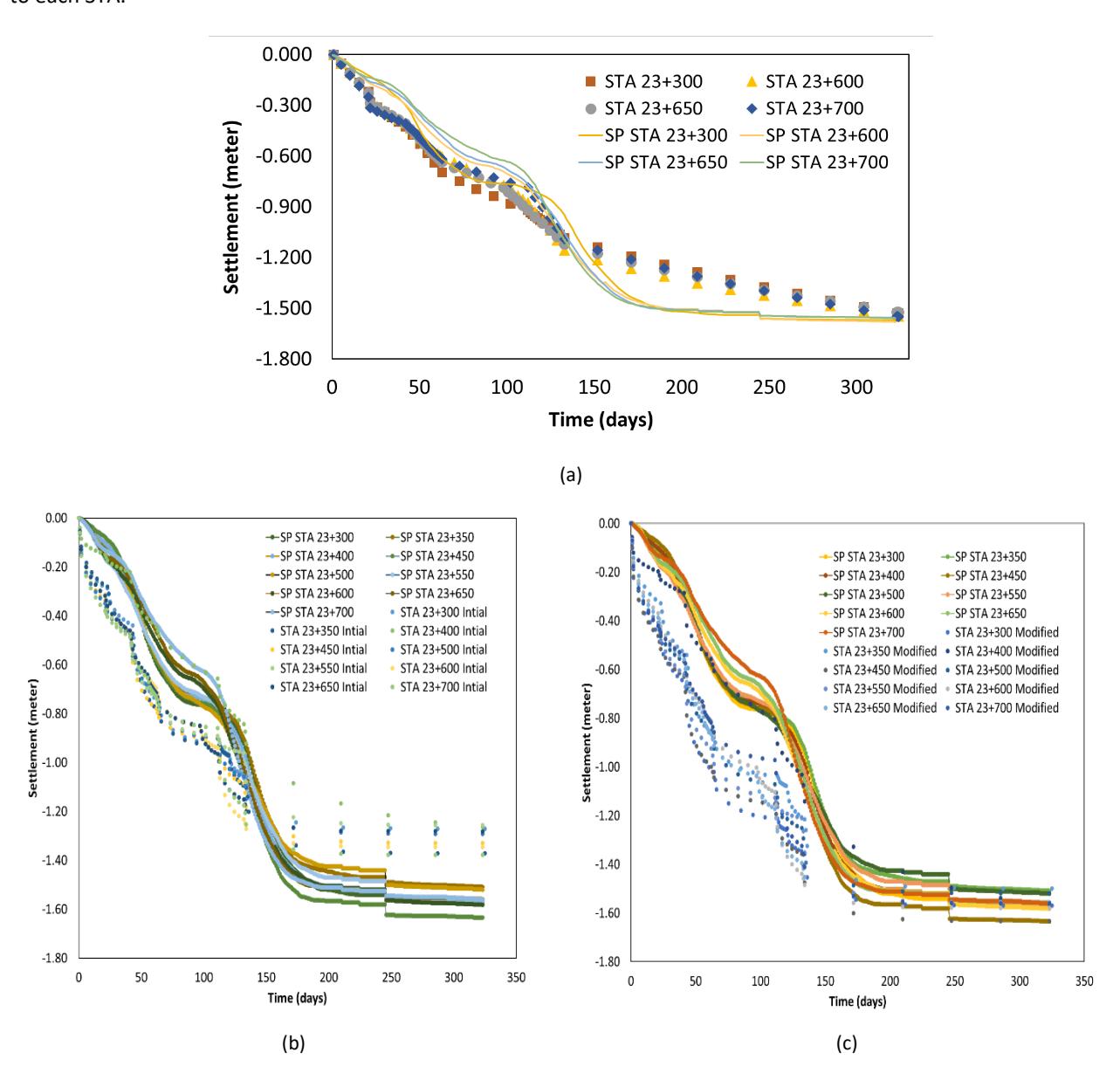
Recapitulation consolidation settlement using values of Cc and Cr at STA 23+300 to STA 23+700 based on: average parameters of the top three (3) soft soil layers (a); before the correction of the Cc and Cr values for nine (9) STAs on the top three (3) soft soil layers reviewed (b); after the correction of the Cc and Cr values for nine (9) STAs on the top three (3) soft soil layers reviewed (c).
Furthermore, in Figure 11 (c) for STA 23+300 to STA 23+700, the consolidation settlement pattern that occurred for 323 days is slightly different from the Settlement Plate. However, in STA 23+400, the consolidation settlement pattern is similar to the settlement plate pattern, asseen in Figure 12. Based on Table 3, STA 23+400 has the smallest embankment stages, 6, and the lowest preloading height, 4.70 meters. This numerical analysis indicates that changes in parameters in different soil layers in the modeling influence the consolidation process despite the final consolidation settlement results being consistent with the data recorded on the Settlement Plate.
Table 8 Final consolidation settlement results at STA 23+300 and STA 23+600 to STA 23+700 using average parameters of the top three (3) soft soil layers.
| CTA | Final Consolidation | Deviation (9/) | |
|---|---|---|---|
| STA | Numerical Modeling | Settlement Plate | Deviation (%) |
| 23+300 | 1.531 | 1.573 | 2.695 |
| 23+600 | 1.547 | 1.582 | 2.231 |
| 23+650 | 1.523 | 1.559 | 2.295 |
| 23+700 | 1.550 | 1.561 | 0.727 |
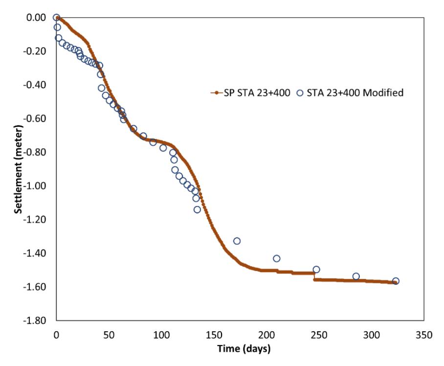
Figure 12 Consolidation settlement using values of C<sub>c</sub> and C<sub>r</sub> modified (correction) at STA 23+400.
The back analysis results of \(C_c\) and \(C_r\) provide more accurate deviation values for the numerical analysis of the final consolidation settlement, indicating that the consolidation parameter values have changed compared to the initial values. The \(C_c\) and \(C_r\) values are consolidation parameters obtained from the oedometer test. However, the oedometer test is time-consuming and expensive, so it is essential to correlate these values with other tests to facilitate the determination of new \(C_c\) and \(C_r\) values for numerical modeling. The consolidation parameter value cannot be separated from the Atterberg Limit parameter in cohesive soil. Terzaghi and Peck (1967) suggested empirical use of the compression index for clay soils whose soil structure is undisturbed, as in Eq. (1). This equation is a linear regression equation. Linear regression is a statistical test applied to a data set to determine and measure the relationship between the variables under consideration. This linear regression usually uses the general equation y = mx + c (Kumari & Yadav, 2018).
In this study, a correlation analysis was performed to examine the relationships between the compression index (\(C_c\)) and the recompression index (\(C_r\)) with the Liquid Limit (LL), as presented in Table 9. The LL value utilized corresponds to the Liquid Limit at the STA, closest to the reviewed STA obtained through the Atterberg Limit laboratory test. The average values for the \(C_c\) and \(C_r\) corrections were calculated based on the average values provided in Table 6 for each STA. For this analysis, the soil type is classified as soft soil, characterized by a Standard Penetration Test (N-SPT) value of 3. The relationships between \(C_c\) and \(C_r\) with LL are expressed in Eqs. (6) and (7), respectively.
\[C_{c} = 0.008(LL) \tag{6}\]
\[C_{r} = 0.002(LL) \tag{7}\] where LL is in percentage (%).
STA Avg. Cc Correction Avg. Cr Correction Liquid Limit (LL) (%) Cc to LL Cr to LL Corr. Factor Avg. Corr. Factor Avg. 23+300 0.920 0.465 84.853 0.011 0.008 0.005 0.002 23+350 0.742 0.216 84.853 0.009 0.003 23+400 0.827 0.252 104.900 0.008 0.002 23+450 0.755 0.273 104.900 0.007 0.003 23+500 0.764 0.202 104.900 0.007 0.002 23+550 0.790 0.226 104.900 0.008 0.002 23+600 0.776 0.180 104.900 0.007 0.002 23+650 0.790 0.197 104.900 0.008 0.002 23+700 0.754 0.164 104.900 0.007 0.002
Table 9 Relationship between Compression Index (Cc) and Recompression Index (Cr) values with Liquid Limit (LL).
The verification of the equation relating the compression index (Cc) and the recompression index (Cr) to the Liquid Limit (LL) is conducted by comparing the corrected LL value with the LL obtained from laboratory testing. As indicated in Table 7, the station at 23+350 exhibits the highest corrected settlement deviation value, recorded at 0.639%. An analysis of the laboratory test data presented in Figure 4 (a) reveals that the average Cc value for stations 23+300 and 23+350 is 0.755. Utilizing the Terzaghi and Peck equation (Eq. (1)), the calculated LL value is determined to be 93.9%. Conversely, for station 23+350, the Cc value derived from numerical correction is reported as 0.742 (see Table 9). The LL value is adjusted to 92.75% when applying the correction factor. Furthermore, at station 23+350, the Cr value is recorded as 0.216, and with the correction factor applied, the LL value is calculated to be 108%. Consequently, this study confirms that the LL value derived from the Cc and Cr corrections equations closely approximates the LL value obtained from the Terzaghi and Peck methodology.
The relationship between the consolidation parameter values based on LL also follows a regression model with independent and dependent variables (Schober, 2018). In the case of Eqs. (6) and (7), the independent variable is the LL value. In contrast, the dependent variable is the consolidation parameter value, which changes according to adjustments made to the final consolidation settlement results. Based on the analysis, this relationship can be applied to soft clay and silty clay soil types in the framework of the accelerated consolidation method using a combination of PVD and Preloading triangle types.
Conclusions
In this study, a settlement has been analyzed numerically based on the field soil parameter data. The results indicate that the numerical analysis underestimates the settlement compared to the observations obtained from Settlement Plates at STA 23+300 to STA 23+700 of the Semarang-Demak toll road. Evaluation using the back analysis method reveals the influence of the compression index (Cc) and recompression index (Cr), which contribute to the magnitude of the final consolidation settlement and help minimize deviation to less than 1%. Additionally, the modeling analysis impacts the settlement pattern and its timing. Furthermore, an empirical equation for the relationship between the compression index (Cc) and the recompression index (Cr) with the liquid limit (LL) was derived: Cc = 0.008 (LL) and Cr = 0.002 (LL), which can be used to estimate the values of Cc and Cr. Obtaining the compression index based on simple soil classification properties, such as the liquid limit, can save time and reduce consolidation test costs.
Acknowledgment
The author wishes to acknowledge the Rector of Universitas Diponegoro for receiving a Universitas Diponegoro scholarship, which provided financial support under grant contract number 144/UN7.A/HK/XII/2022. Moreover, the authors are grateful to MIDAS Information Technology Co., Ltd. and PT. Midasindo Teknik Utama is responsible for granting the Midas GTS NX software license. They also extend their gratitude to PT. PP Semarang Demak, a PT PP (Persero) Tbk subsidiary, is responsible for supporting and providing the essential data required for this paper. The authors are deeply appreciative of this assistance. Additionally, they would like to thank Muhamad Reiyhan Putra Arvie and Rizza Muhammad Shan for their valuable and insightful discussions throughout this study.
Compliance with ethics guidelines
The authors declare they have no conflict of interest or financial conflicts to disclose.
This article contains no studies with human or animal subjects performed by authors.