
Introduction
Approximately 1.3 million individuals are perishing annually in global traffic accidents, while the number of injuries ranges between 20 and 50 million. Therefore, the International Status Report on Road Safety has examined road safety conditions in 178 nations using survey data (WHO, 2022). Based on the WHO report, injury-related deaths constitute the primary cause of mortality for individuals between the ages of 5 and 29. This suggests that traffic injuries persist as a substantial public health issue, which is prevalent in low and upper-middle-income nations, such as China. From 2016 to 2019, there has been a substantial rise in the frequency of traffic collisions and fatalities in China, with 256,101 injuries and 62,763 deaths recorded in 2019 (Statista, 2023). Consequently, drivers using these routes must exercise extra caution and adhere to safety measures.
Previous research reported that specific trends occurred in 2022 about the causes of accidents. The predominant elements contributing to these accidents are drowsiness, distracted driving, alcohol-related incidents, and excessive speeding (Kaur & Sobti, 2018; Rahman et al., 2020; Raveena et al., 2020; Song et al., 2019). The speed of a vehicle is a crucial factor in determining the extent of damage caused by a collision. However, driving at high velocity does not invariably entail risk if the driver is dependable (Alasmari et al., 2023; Q. Liu et al., 2021; Pranoto et al., 2023). Ensuring road safety includes determining the appropriate speed limit based on the conditions of the driver and the car. Insufficient driver alertness hampers the ability to react promptly and avert a catastrophe while driving at high velocities. Furthermore, increased distractions and speed significantly amplify the risk of an accident or collision, leading to severe damage or fatality. To address this risk, the Advanced Driver Assistance System (ADAS) has been designed as a current and future in-vehicle technological system aimed at improving driving safety (Cicchino, 2017; Nandavar et al., 2023; Spicer et al., 2018).
ADAS can effectively decrease the probability of a collision and mitigate the extent of injuries sustained in the event of a crash. According to (Phan et al., 2023; Xu et al., 2023), forward collision warning systems yielded a 27% decrease in frontto-rear crashes, and autonomous emergency braking systems with low-speed capabilities caused a 43% reduction. The results showed that using automated emergency braking systems operating at low speeds and systems could decrease front-to-rear collisions by half. (L. Yue et al., 2018) discovered that methods for warning of forward collisions caused a 35% reduction in accidents during foggy conditions. This showed the significance of enhancing ADAS technology in society, demonstrating the favorable influence of ADAS-equipped automobiles on road safety. However, most ADAS that rely on visual detection often use cameras. This suggests the inability to immediately anticipate the cognitive and mental state of the driver, leading to a delay in system response.
Compared to ADAS, an Electroencephalogram (EEG) is a highly effective device for monitoring the status of a driver. It directly measures cognitive abilities and mental state by capturing signals from the human brain (Li et al., 2022; Romahadi et al., 2024; Xia et al., 2023; Zhang et al., 2023). Furthermore, the high temporal resolution enhances the EEG signals to capture neural activity in the driver's brain. Chen et al. (Chen et al., 2024) used spectral graph convolutional networks to diagnose mental weariness. (Y. Yang et al., 2021) proposed a new comprehensive learning system based on a large deep convolutional neural network (CNN) to detect fatigue using EEG. (Feng et al., 2025) also proposed a pseudo-label-assisted subdomain adaptation network with coordinated attention for detecting driver fatigue based on EEG. Several investigations use the deep learning method and Power Spectral Density (PSD) feature for fatigue detection (Apicella et al., 2022; Chen et al., 2021; Jantan et al., 2022). However, previous research has fully used spectral domain features without eliminating redundant features. Complex CNN models have also been applied to overcome feature redundancy, increasing the computational cost. Therefore, this research aimed to implement a lightweight CNN architecture to classify multi-class driver fatigue. The EEG was transformed into PSD, followed by a statistical method to diminish the feature dimensionality. A total of two feature ranking algorithms, Chi-square and Relief feature (ReliefF), were used to identify significant features. This study also proposed a classification method that used a lightweight CNN model and effectively reduced several redundant features, serving as a suitable option for real-world applications.
Materials and Methods
The process of determining the state of alertness using EEG data consists of four distinct stages and primarily relies on the CNN model. First, the raw EEG data passes through the pre-processing stage that tries to eliminate noise in the original signals. These signals are standardized to mitigate the impact of variances in magnitude and range of values across distinct measurements. Second, statistical combinations of Power Spectral Densities (PSDs) are extracted from different frequency bands. Third, feature augmentation is implemented using the Synthetic Minority Over-sampling Technique (SMOTE) method. Fourth, a feature selection algorithm is used to reduce the importance of irrelevant variables. Feature selection entails using the Chi-square and ReliefF algorithm methods, specifically developed to enhance classification accuracy and reduce learning time.
Dataset
Comprehensive experiments are conducted on publicly available datasets to assess the efficacy of the proposed method. The SEED-VIG dataset, which consists of EEG data collected during driving tasks, is a locally shared proprietary dataset. Zheng and Lu developed and provided the SEED-VIG data (Zheng & Lu, 2017). Using a driving simulation platform, the dataset includes EEG, electrooculogram (EOG), and eye movement data from 23 participants. A road scene is depicted on a liquid crystal display (LCD) screen before the modified vehicle, showing real-life conditions, as presented in Figure 1. The driving simulation uses virtual reality technology to recreate a variety of vehicles, weather conditions, and road arrangements, as shown in Figure 1. Neuroscan technology is synchronized to record forehead EOG, EEG, eye movements, and eye-tracking glasses. Driving simulation examinations are conducted on physical cars whose engines and other extraneous components have been removed. The participants were instructed to operate the vehicle, applying pressure to the gas pedal and steering wheel during the test. The driving scenario was updated simultaneously according to the actions performed by the participants without receiving any warning feedback after sleep.
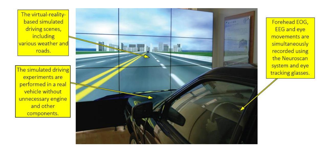
Figure 1 Driving simulation scenarios.
Figure 2 Placement of electrodes for EEG measurement.
The participants were instructed to operate the vehicle, applying pressure to the gas pedal and steering wheel during the test. The driving scenario was updated simultaneously according to the actions performed by the participants without receiving any warning feedback after sleep. The linear and repetitive nature of the testing environment causes fatigue or sleepiness. The Neuroscan ESI measurement equipment can obtain EEG and EOG signals at a sampling rate of 1000 Hz. The EEG cap consists of a total of 64 electrodes, which are strategically placed on the scalp according to the internationally recognized 10-20 system. The EEG function in this study recorded 17 EEG channels, consisting of 11 posterior EEG channels and 6 temporal EEG channels. Posterior EEG channels include 'FT7', 'FT8', 'T7', 'T8', 'TP7', 'TP8', 'CP1', 'CP2', 'P1', 'P2', 'P2', 'P03', 'PO2', 'P04', 'O1', 'O2', and 'O2' as shown in Figure 2. Additionally, the dataset includes a 4-channel forehead EOG for further analysis.
\[PERCLOS = \frac{blink + CLOS}{interval}\] \[interval = blink + fixation + saccade + CLOS\] (1)
EEG signals from 11 channels were recorded in the posterior region marked in yellow, while signals from 6 channels were in temporal locations shown in blue. SMI Eye Tracking Glasses 2 has an infrared camera capable of capturing eye gaze and various eye movements such as eye blinks (CLOS), saccades, and fixations. The labels assigned to the data set correspond to the PERCLOS (Percentage of Eyelid Closure) levels observed by the eye tracker, as indicated by Eq. (1).
| Filenames | Subject Number | Number of Samples | ||
|---|---|---|---|---|
| Awake | Tired | Drowsy | ||
| '5_20151012_night.mat' | S05 | 422 | 304 | 159 |
| '7_20151015_night.mat' | S07 | 98 | 753 | 34 |
| '9_20151017_night.mat' | S09 | 208 | 636 | 41 |
| '11_20151024_night.mat' | S11 | 324 | 545 | 16 |
| '14_20151014_night.mat' | S14 | 225 | 464 | 196 |
| '15_20151126_night.mat' | S15 | 289 | 525 | 71 |
| '16_20151128_night.mat' | S16 | 202 | 177 | 506 |
| '20_20151129_night.mat' | S20 | 625 | 50 | 210 |
| Total | 2393 | 3454 | 1233 | |
Table 1 The dataset used in this study.
Furthermore, participants were classified as awake when their PERCLOS value was less than 0.35 and considered sleepy when their value exceeded 0.7. Several participants, particularly between 0.35 and 0.7, showed signs of fatigue through annotations.
The driving task was completed with 23 participants in the study, although some reports lacked sufficient or complete data on specific psychological problems. Certain participants demonstrated inadequate sampling of driving conditions, leading to significant data imbalance and limited effects. Therefore, samples considered for use in this experiment were obtained at night. In addition to increasing the efficiency of signal processing time, the sample size that had complete classes only in the night experiment was measured from eight participants. The aggregate for each selected participant consisted of 2393 awake, 3454 fatigue, and 1233 drowsy segments. The overall sample size for the six participants consisted of 7080 segments, as shown in Table 1. The EEG sample of one participant is contained in one file, with a number indicating each name before the filename.
Preprocessing of Raw EEG
The classification was implemented on a 64-bit Windows 11 operating system, an RTX 4080 super graphics processing unit, and a 14th-generation Intel Core i9 central processing unit. Calculations were carried out using MATLAB software version 2023b. EOG signals present in the unprocessed EEG data were ignored. Raw EEG data were processed using a band-pass filter ranging from 1-75 Hz to exclude extraneous signals that did not originate from the brain. A bandpass filter with a 1-75 Hz frequency range was used. A notch filter removed signals with a frequency of 50 Hz originating from an electric current. Subsequently, the average EEG signal across electrodes was calculated and applied to each time point from the signal at every electrode. This effort aimed to produce a reference characterized by a lack of noise or electrical charge. Fundamental signal modifications were performed to reduce the influence of significant variance in the EEG signal that exceeded acceptable thresholds. The EEG signal was passed through baseline correction by subtraction of the baseline period average value of each time point at the baseline and post-stimulus intervals.
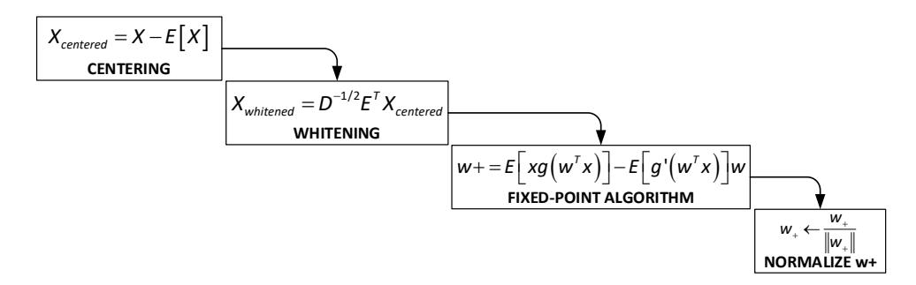
Figure 1 FastICA algorithm.
The EEG signal has been pre-filtered to remove extraneous noise. However, internal artifacts originating from the individual, such as eye blinks, heartbeats, and muscle movements, have not been filtered out (Jiang et al., 2019; Khatun et al., 2016). Artifact filtering is essential to effectively remove unwanted noise from EEG data. Independent Component Analysis (ICA) characterizes the components that make up the EEG signal. In this research, the FastICA method was used (M. Yue et al., 2022), with the computation stages shown in Figure 3. FastICA is derived from optimizing the components' non-Gaussianity, quantifying their statistical independence. The algorithm is renowned for its superior efficiency and rapidity compared to alternative ICA. In the process of centering, the average value is subtracted from each variable to ensure that the data has a mean of zero. During the whitening process, the data is altered for the different components to become uncorrelated and have a variance of one. The eigenvalue decomposition to determine the variance in the concentrated data yields the values E and D. This process is often carried out using Principal Component Analysis (PCA). Popular options include kurtosis or negentropy when selecting a measure of non-Gaussianity due to its greater resilience. Subsequently, an iterative fixed-point method is used to optimize the selected non-Gaussian metric. The Independent Component Label (ICLabel) method will identify components that do not originate from the brain (Pion-Tonachini et al., 2019). Once the EEG signal is effectively free of any artifacts, it is divided into segments of eight seconds duration.
Feature Extraction
After the noise and artifact cleaning process, EEG signals are decomposed into five types of brain frequencies, including delta (1–3 Hz), theta (4–7 Hz), alpha (8–12 Hz), beta (13 –30 Hz), and gamma (31–75 Hz) using finite impulse response (FIR) filtering function. This is followed by Welch's method to convert brain signals from the temporal to the frequency domain (Gupta et al., 2021; S. Liu et al., 2023). For a continuous signal over time, the PSD present for the stationary process must be determined. This explains how the amplitude or time series of the signal is distributed over the frequency. Moreover, the amplitude represents either the actual physical power or, more commonly used to conveniently describe abstract signals characterized by the square value. Eq. (2) is the main formula for calculating PSD (Gupta et al., 2021; S. Liu et al., 2023).
\[S(e^{jw}) = \frac{1}{2\pi N} \left| \sum_{n=1}^{N} x_n e^{-jwn} \right|^2\] (2)
Finite time series with \(1 \le n \le N\), for example, data collected at periodic intervals \(xn = x(n\Delta t)\), up to the end of the measurement term \(T = N\Delta t\). generalize the definition of PSD straightforwardly. Statistical functions and four types of energy bands are applied to Welch's computational results. These statistical functions include mean, standard deviation, median, minimum, and maximum values. The four energy ratios are shown in Eqs. (4)-(7) (Al-Qazzaz et al., 2021). Dimensionality reduction is also achieved through statistical and energy functions, with the energy of each band computed using Eq. (3).
\[E = \sum_{n=1}^{N_{PSD}} \left(\frac{F(n)}{N_{PSD}}\right)^2 \tag{3}\]
\[R_1 = \frac{(E_\theta + E_\delta)}{E_\beta} \tag{4}\]
\[R_2 = \frac{E_{\gamma}}{E_{\delta}} \tag{5}\]
\[R_3 = \frac{E_\beta}{E_\alpha} \tag{6}\]
\[R_4 = \frac{E_\alpha}{E_\theta} \tag{7}\]
F(n) denotes the signal's output at a specific frequency n. The feature extraction process culminates in balanced results for each class during the training phase. Based on the number of samples between classes that are not the same, the sample is multiplied using the SMOTE algorithm (Wang et al., 2024), as shown by Eq. (8). Where x is the original sample, r is a random number between 0 and 1, j is between 1 and the nearest sample number, and z is the closest sample.
\[x_i' = x_i + r \times (z_{ij} - x_i) \tag{8}\]
Selecting the Importance Feature
Chi-square is a statistical method to select the most significant features from a dataset. This is especially useful in categorical data analysis when determining which features have the most substantial relationship with a particular target variable (Teng & Bi, 2017). Chi-square statistics are calculated for each feature in the EEG dataset, as shown in Eq. 9. This statistic measures the dependency between a feature and a target variable based on the difference between each category's observed and expected frequencies within the feature.
\[\chi^2 = \sum \frac{(O_i - E_i)^2}{E_i} \tag{9}\]
\(O_i\) is the discovered occurrence rate for category i and \(E_i\) is the expected frequency for category i. For the test of independence, the expected frequency for each cell in a contingency table is calculated using Eq. (10).
\[E_{ij} = \frac{(Row\ Total)_i \times (Column\ Total)_i}{Grand\ Total} \tag{10}\]
The computed chi-square is compared with the level of significance, which is determined by the selected confidence level of 0.05. When the computed statistic is greater than the significance level selected, the null hypothesis, showing that there is no relationship between the feature and the target variable, is rejected. Features with Chi-square statistics exceeding the critical value are considered significant and sorted by importance. The most significant is in the first column, and others have lower importance, indicating a strong relationship with the target variable.
Relief Feature Selection (ReliefF) is a popular and effective feature selection algorithm mainly used for supervised classification tasks (L. Yang et al., 2021). ReliefF starts by initializing the weights for each feature to zero. This is followed by identifying the closest features from the same class and examples from different courses in the iteration process. When the value of the current feature is the same as the nearest class, the weight will be increased. However, the weight is reduced when the current value of a feature is different from the value of the nearest class. The magnitude of the weight change depends on the difference between the feature's current value and its closest neighbors, as shown in Eq. (11). Updating the weight W[A] for each A based on the difference in feature values R and its near-hits and near-misses.
\[W[A] = W[A] - \sum_{H \in Hits} \frac{(A(R) - A(H))^2}{mk} + \sum_{M \in Misses} \frac{(A(R) - A(M))^2}{mk}\] (11)
where m is the number of classes and k is the number of neighbors. After repeating all the calculations in the dataset, ReliefF ranks the features based on their weights. Features with higher weights are considered more important for the classification task.
\[Accuracy = \frac{TP + TN}{TP + TN + FP + FN}\] \[Sensitivity \text{ (Re call)} = \frac{TP}{TP + FN}\] \[Precision = \frac{TP}{TP + FP}\] \[Specificity = \frac{TN}{TN + FP}\] \[F-score = \frac{2TP}{2TP + FP + FN}\] (12)
Classification
Several feature sets were selected based on the significance analysis results of Chi-square and ReliefF. To assess the efficacy of various variables in detecting driver attention, a series of experiments were carried out using deep learning methods, specifically a CNN-type neural network, as shown in Figure 4. In CNN, the input layer is the first layer that uses features extracted from five types of statistical values calculated from the PSD. The input feature is in vector form with dimensions 1*493. The next stage includes four convolution layers with different filter dimensions. After passing through all the convolution stages, Global Average Pooling overcomes the problem of reducing the spatial dimension of the feature map while increasing the depth, leading to excessive adjustments. Each neuron in the fully connected layer is related to every neuron in the layer below. The output of each neuron in the last layer is multiplied by the weight and summed with the bias before being passed through the activation function. The final stage uses the SoftMax function to convert an arbitrary real value vector into a probability, each element in the range [0, 1], and the sum of all elements equals 1. The classification process repeats for 100 epochs. To ensure reliability, the final result is achieved by calculating every trial using selected features. A total of two classifications, namely intra-subject and cross-subject, were performed. Intrasubject classification uses data from the same subject for training and testing. Meanwhile, cross-subject classification combines all data from four subjects, followed by randomization. Before the training, the statistical variation features of the PSD values in each frequency band are randomly partitioned into a training set, subjected to 20% hold-out validation testing, as shown in Figure 5. The model performance results are analyzed using characteristics such as accuracy, precision, recall, specificity, and F-score, as shown in Eq. (12). When the actual value and the prediction are positive, it is called a true positive (TP). However, when the actual value and the prediction are negative, it is called a true negative
(TN). A false positive (FP) is obtained when the truth is negative but the prediction is positive, also called a type 1 error. When the truth is positive but the forecast is negative, it is called a false negative (FN), also recognized as a type 2 mistake.
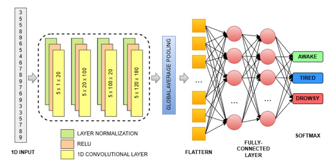
A lightweight CNN model architecture.
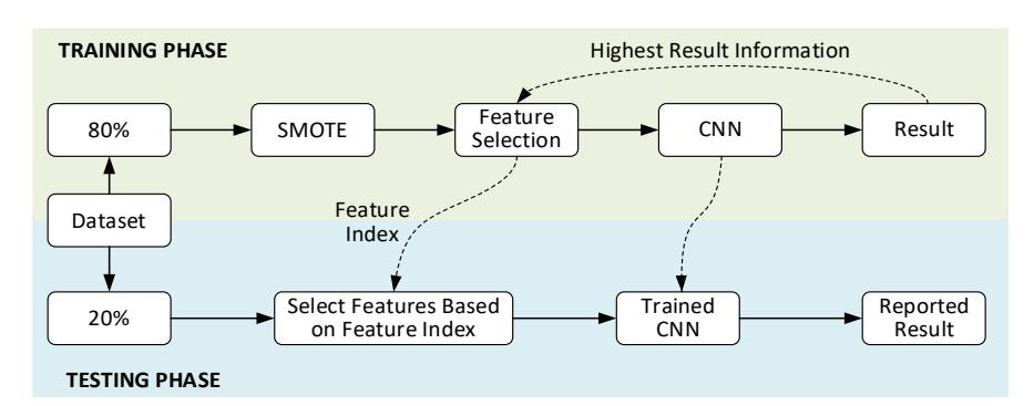
Illustration of data division during the classification process.
Result
Class Label Distribution Analysis
The fatigue index of some individuals is distributed centrally without outliers, but there is also a large amount of unbalanced data, as shown in Figure 6. The class with the most significant sample shows the fatigue condition among the three classes. Only S16 data for the fatigue index is centered on the drowsy and S20 on the alert conditions. Datasets S05, S14, S15, and S16 show an even distribution of samples, forcing their selection for further investigations. An unbalanced sample size significantly affects the effectiveness of the classification model. The model trained with imbalanced data may be biased towards the majority class due to their optimization to reduce total error. This suggests that the model can predict mostly the majority class, although the examples come from the minority class. Imbalanced data is capable of causing suboptimal generalization performance, making it difficult for the model to classify instances belonging to the minority class accurately. To address the limitation, oversampling is a powerful method to overcome disparity between classes in classification tasks. This includes increasing the proportion of minority-class samples to achieve a balanced class distribution in the dataset.
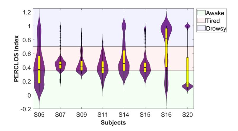
PERCLOS index distribution.
Results of Feature Selection
A subset of related characteristics from the initial feature set is selected to improve model performance or decrease computational complexity. Feature selection aims to eliminate redundant, repetitive, or performance-degrading characteristics while retaining the most discriminative and informative features. The selection of the most pertinent attributes can reduce the dimensionality of data, leading to more straightforward, easier-to-understand models and faster computation. However, original features are retained when the removal process causes a loss of accuracy. Figure 7 shows the feature selection results using the Chi-square and ReliefF algorithms. A total of 493 features are divided into 20 groups, selecting from the lowest numbers 5 to 493 with intervals of 5% for each level, based on the computational output of the ranking algorithms. The graph shows that the accuracy decreases considerably when extraneous features are removed based on Chi-square and ReliefF. As the number of features increases, the minimum accuracy value also increases. With 366 features, the Chi-square algorithm selection has the highest accuracy, and ReliefF achieved the greatest at 390 features. Moreover, the number of features does not suggest that the composition of each subject is the same. Chi-square has the highest accuracy in the training phase. Validation of both algorithms based on the features that produce the highest accuracy is needed for the testing phase to determine the best.
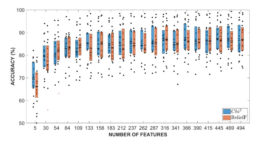
Comparison of feature selection results.
CNN Performance on Intra- and Cross-Subject Classification
Intra-subject classification is a machine-learning task that aims to classify data samples from the same individual. In this research, intra-subject classification is used by analyzing data from the same individual to make predictions or diagnose problems. This method consists of examining data from each subject independently rather than pooling data from multiple subjects. Furthermore, it recognizes that individuals can show patterns or properties in their data to achieve correct classification or predictions. Lightweight CNN is used in categorization, and the results are compared to determine the most accurate feature. The results of CNN classification for each subject based on Chi-square and ReliefF are shown in Figure 8. In the classification, training is carried out on samples in each subject, divided into 80% as training and 20% as testing. A total of two iterations are applied during the process, each with a different distribution of divisions in the training and testing stages. To verify that the selected features are optimal, each feature from the individual algorithms is applied in every iteration. The selection of the best feature algorithm is based on the highest accuracy results. Based on the classification results, Chi-square produces an accuracy of 70.87% and ReliefF of 71.01%. The confusion matrix, as presented in Figure 9(a), highlights that the CNN model maintains a performance level exceeding 60% even when applied to cross-subject classification.
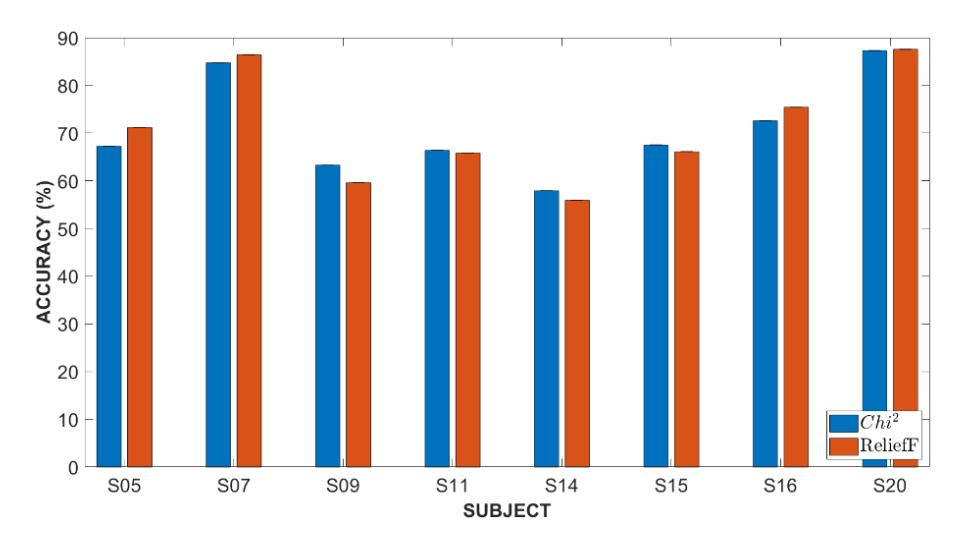
Accuracy rate of each subject with different feature selection algorithms.
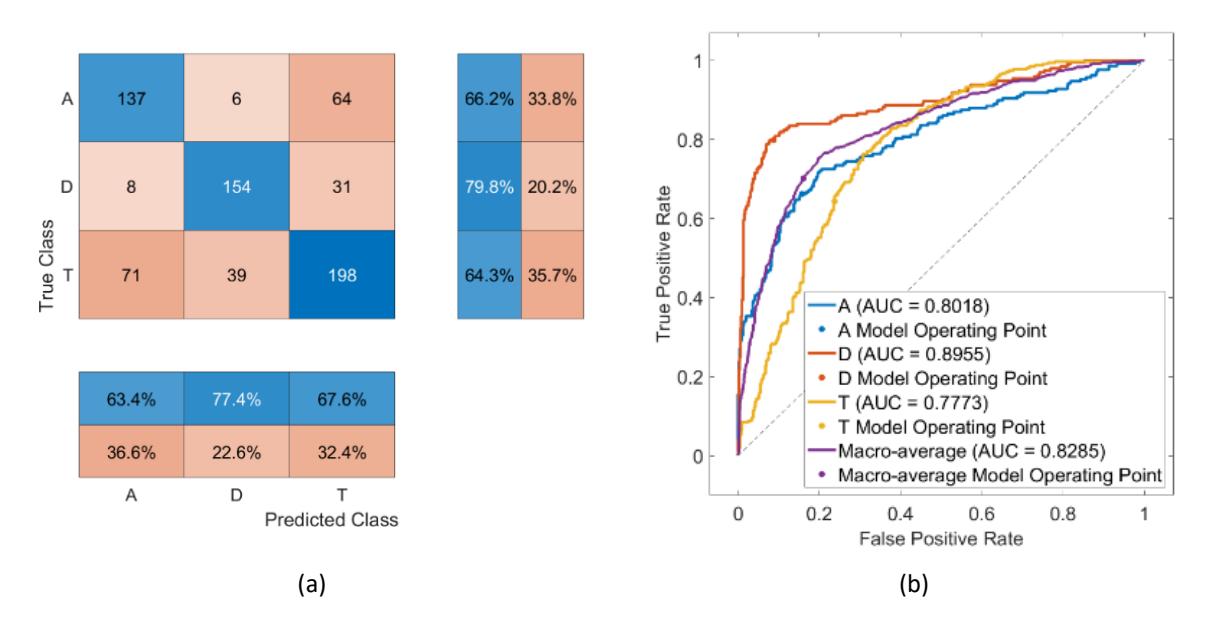
Cross-subject confusion matrix (a) and ROC curve (b).
This is notable given that cross-subject classification involves using data from subjects different from those on which the model was trained, which introduces greater variability in the data distributions. In this scenario, the dataset is composed of data from four different subjects, and the total dataset is divided into 80% for training and 20% for testing.
This division ensures that the model is trained on a sufficiently large and varied dataset while also being evaluated on a separate subset to assess its generalization ability. The classification process involves running the CNN model for 100 epochs in both intra- and cross-subject classification tasks. The choice of 100 epochs strikes a balance between allowing the model to learn meaningful patterns from the data and avoiding overfitting. The performance of the model is monitored through the confusion matrix, where the box highlighted in blue indicates the number of samples that were successfully and correctly classified by the CNN. This visual representation provides insight into how well the model is able to generalize across subjects with differing data distributions. Despite the inherent challenges of cross-subject classification, where the distribution of features may vary significantly, the CNN still manages to achieve a reasonably high classification accuracy, demonstrating its robustness and effectiveness in handling such variability.
| Class | |||
|---|---|---|---|
| Parameter | Awake | Tired | Drowsy |
| True Positive | 137 | 198 | 154 |
| False Positive | 79 | 95 | 45 |
| False Negative | 70 | 110 | 39 |
| True Negative | 422 | 305 | 470 |
| Precision | 0.6343 | 0.6758 | 0.7739 |
| Sensitivity | 0.6618 | 0.6429 | 0.7979 |
| Specificity | 0.8423 | 0.7625 | 0.9126 |
| Accuracy | 0.6907 | 0.6907 | 0.6907 |
| F-score | 0.6478 | 0.6589 | 0.7857 |
Table 2 Cross-subject classification performance.
The box in blue shows the number of samples successfully and correctly classified by the CNN. Detailed values and percentages of CNN performance from calculating the confusion matrix are shown in Table 2. Based on classification, the best and weakest performance are obtained when the CNN faces data labeled as drowsy and tired, respectively. The results showed that the overall accuracy value of the model was 69.07%. The best value for the specificity parameter was achieved across all classes compared to other parameters, as supported by the receiver operating characteristic (ROC) curve shown in Figure 9(b). The ROC curve shows the performance of CNN in classifying each class at various classification thresholds. On the y-axis of the ROC graph is the actual positive rate (sensitivity), while the x-axis represents the FP rate (1 minus specificity). The percentage of erroneous positives of adverse events is misclassified, while sensitivity indicates the proportion of positive events that are accurately classified. This graphic proves that CNN can detect each class accurately, with an average area under the curve (AUC) value of 82.85%. As shown in the specificity parameter in the confusion matrix, CNN is most accurate when detecting samples labeled as drowsy, with an AUC value close to 90%. The specificity of this test measures the ability to correctly identify drivers who are not drowsy, alert, or tired. This test is particularly designed to produce a few FP results.
Discussion
The results indicate that the CNN model performs significantly well, even with relatively simple data input, highlighting its robustness. This performance, however, also reveals an important observation: each brain signal exhibits unique characteristics across different subjects. This is evidenced by the noticeable variation in classification results, which differ substantially between subjects. While the CNN model successfully recognized well-trained data in several subjects, the accuracy dropped below 70% in subject S14. This decline in performance aligns with previous research, which has highlighted the limitations of EEG signals, particularly their dynamic nature, which varies significantly depending on the subject and time. The classification process, both intra- and cross-subject, aims to generalize across these variations by collectively classifying data samples from multiple individuals or subjects.
The comparison between intra- and cross-subject classification reveals a key challenge: cross-subject classification accuracy is generally lower. This discrepancy is common in multi-class cross-subject classification, as many studies report lower accuracy when classifying EEG signals across different individuals. The primary reason for this is the inherent variability in EEG characteristics over time and between individuals. While several previous models utilizing the SEED-VIG dataset have reported higher accuracy than the CNN model used in this study, it is essential to consider the differences in model complexity, number of classes, and testing methodologies. For instance, Cui et al. (2022) achieved 73.22% accuracy in cross-subject classification using a more complex and interpretable CNN. In another example, Paulo et al. (2021) reached 75.87% accuracy by applying deep CNN techniques for binary classification. Meanwhile, Shen et al. (2021) used PSD features combined with an SVM, yielding an accuracy of 62.51% in inter-subject classification.
Despite these differences, the model in this research offers competitive results, especially considering the simplicity of the approach and its potential for real-time applications. In comparison to previous studies, this CNN model demonstrates strong performance in both intra- and cross-subject classification tasks, providing valuable empirical evidence for its
viability in real-time EEG-based applications, where classification accuracy and robustness across varying subjects are crucial.
Conclusion
In conclusion, this research evaluated the multi-class detection system for driver fatigue levels using EEG. The raw data of the EEG were obtained from the public dataset and analyzed through preprocessing, feature extraction, feature selection, and classification using a lightweight CNN. Feature extraction from five types of frequency bands used the Welch method, which produced a PSD-type frequency domain. Each frequency band in PSD form was re-extracted using five types of statistical calculations and four types of energy bands to obtain 493 features. The optimal features were selected through the ReliefF test with the highest accuracy value. A CNN-type classification model was built using four convolution layers. Each convolution layer was supported by ReLU activation and normalization functions, connected to a multi-layer neural network with three class outputs. After training for 100 epochs, the lightweight CNN recognized the test data accurately. The average accuracy value for intra-subject classification was 71.01%, while the cross-subject classification had 69.07%.
Acknowledgments
The authors are grateful to Universitas Mercu Buana for the financial assistance received under contract No. 02-5/215/B-SPK/II/2024.
Compliance with ethics guidelines
The authors declare they have no conflict of interest or financial conflicts to disclose.
This article contains no studies with human or animal subjects performed by authors.