
Introduction
Compliant mechanisms were developed based on the elastic deformation of flexible joints, resulting in compact and simplified structures. However, their working range was limited due to structural constraints. To overcome this, adjustments in the size and design of flexure hinges were required. In response, various compliant mechanisms were proposed, designed, and fabricated in previous studies to expand the workspace while retaining the benefits of simplicity and precision. The displacement amplification ratio (DAR) of the lever-type flexure hinge was enhanced thanks to the rotational center of the flexible hinge (Huang & Shen, 2022). The experimental test confirmed the results with a 2.49% error, which was comparable to the FEM. The stiffness model proposed by (Zhang & Yan, 2024) was used to adjust the stiffness of the compliant mechanism. The experimental test and finite element method results were consistent with the proposed model. The fast tool servo introduced by (Paniselvam et al., 2023) aimed to improve ultraprecision machining performance. To enhance the DAR of the microgripper, shape memory alloy was proposed with the aid of the pseudo-rigid body model. The experimental and model results achieved a force-bearing capacity ranging from 0.152 to 0.381 N. The column bending test and the four-point bending test conducted by (Meyer et al., 2023) were carried out to test deflection. The experimental results showed deflection ranging from 0.4 mm to 1 mm.
Faculty of Mechanical Engineering and Technology, Ho Chi Minh City University of Industry and Trade, 140 Le Trong Tan, Tay Thanh Ward, Ho Chi Minh City 700000, Vietnam
Faculty of Fundamental Sciences, PetroVietnam University, Ho Chi Minh City 700000, Vietnam,
Faculty of Mechanical Engineering, Industrial University of Ho Chi Minh City, 12 Nguyen Van Bao Street, Hanh Thong Ward, Ho Chi Minh City 700000, Vietnam
The hybrid flexure hinge, designed using elliptical and hyperbolic shapes by (Wang et al., 2024), showed better performance than both the elliptical and hyperbolic flexure hinges. A new design of the notch flexure hinge was proposed by (Wei et al., 2023) by modifying the elliptical cross-section. The experiment confirmed the performance of the new model. The working range of 28.7 µm × 27.62 µm for a two-degrees-of-freedom (DOF) compliant positioning stage (Wu et al., 2024) was obtained through experimental testing. This result was consistent with the finite element model. Similarly, the two-DOF compliant positioning stage (Sun & Hu, 2024) achieved a working range of 28.27 µm × 27.62 µm as confirmed by experimental testing, and the results agreed well with the finite element analysis. he stiffness model and finite element model developed by (Shi et al., 2024) were applied to minimize parasitic shifts in a flexurebased motion-decoupled XYZ stage with a quasi-symmetric 3-Prismatic-Prismatic-Prismatic structure. The experimental testing results validated the outcomes of the models. A compound amplifier (Das & Shirinzadeh, 2024) was implemented to improve the working range of the microgripper compliant mechanism. The experimental testing showed a high DAR of 34.5 times, consistent with the FEM results obtained using ANSYS. The DAR of a nonlinear singlestage compliant orthogonal displacement amplifier was determined through both experimental testing and FEM by (Chen et al., 2024). The results from both models showed good agreement. The stress in a semi-circular notch flexure hinge (Meng et al., 2023) was determined using the finite element method and Castigliano's second theorem. The experimental results aligned well with those from the two proposed models. The transfer matrix method based on Timoshenko beam theory (Ling et al., 2023) was applied to determine displacement and stress in the notch flexure hinge. The experimental results indicated that the proposed model achieved high accuracy.
A significant improvement in the displacement of low-stress flexible hinges (Abedi et al., 2023) was achieved using a method involving two-way symmetrical cutting and the principle of differential leverage amplification. The finite element method confirmed an improvement of 2243%. An S-shaped flexure hinge was proposed for the bridge-levertype mechanism (Wu et al., 2022). Both the FEM and matrix-based compliance modeling were used to determine a DAR of 5.3 times, and experimental results confirmed this finding. The bridge-type compliant displacement mechanism and the Scott-Russell mechanism were applied in a compliant XY micro-positioning stage (Lyu & Xu, 2022) to increase the working range of the proposed design. The FEM and experimental results showed a working range of 181.0 μm × 179.5 μm, with resonance frequencies of 178 Hz and 248 Hz in the x and y directions, respectively. The optimal microgripper compliant mechanism (Zhang et al., 2021) was designed using the response surface method. Both FEM and experimental testing confirmed a DAR of 548.42 μm and a resonant frequency of 334 Hz. The combination of S and J layers to create an asymmetric stiffness pattern, along with Castigliano's second theorem and FEM, was used by (Marathe et al., 2021) to determine the angular output and performance of a precision motion stage compliant mechanism. The experimental results validated the proposed models. Finally, a bridge and lever-type compact compliant mechanism (Das et al., 2020) was applied in micro-positioning systems to amplify motion by 6.5 times using the pseudo-rigid body model. The results were confirmed through both experimental testing and finite element analysis.
Previous studies mostly built algorithms and experiments to determine the stress and displacement of the compliant mechanism amplifying flexure hinge. However, these methods are very difficult, and the results are not high, even expensive. In these studies, a simpler and less expensive method is proposed but still ensures reliability as follows:
- 1. Using elastic joints, we performed a finite part analysis in ANSYS to estimate the stress and displacement of the amplification ratio compliant mechanism.
- 2. Using the Taguchi method to design 27 experiments with 27 models with different design variable sizes designed with SolidWorks software
- 3. To select a model with high displacement amplification but still ensure the strength of the mechanism's ability to work effectively, multi-criteria decision-making methods such as the EAMR method, SAW method, WASPAS method, and EDAS method have been applied.
- 4. Methods such as Taguchi, interaction analysis, variance analysis, and 3D surface graph analysis have been applied to determine the reliability of the proposed methods.
The selection of four multi-criteria decision making methods aims to have more evidence to confirm the optimal case. This helps increase the reliability of the research results. Because all four methods confirmed a consensus on one optimal case. In addition, the Taguchi method also proves that the results of the four optimization methods are reliable.
Design and Analysis of Amplifying Compliant Mechanism Flexure Hinge
Design an Amplifying Compliant Mechanism Flexure Hinge
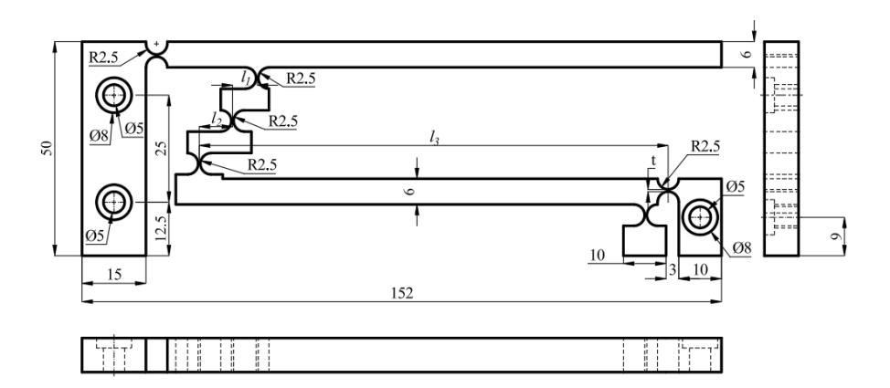
An amplifying compliant mechanism flexure hinge was applied in the Gas-Liquid Thermoelectric Power Device, as depicted in Figure 1. The overall dimensions of the model were 128 mm × 50 mm × 8 mm. The design dimensions and design variables of the model were illustrated in Figure 2. The proposed mechanism model was designed using SolidWorks software. A total of 27 models with different values for the design variables were created based on the experimental design results obtained using the Taguchi method.
The selected model's design variables included the thickness of the flexure hinge and three distance dimensions between the flexure hinges. The thickness of the flexure hinge, denoted as t, varied across three levels: 0.3 mm, 0.4 mm, and 0.5 mm. The first distance between two flexure hinges, denoted as l₁, varied at three levels: 5.2 mm, 5.5 mm, and 5.8 mm. The second distance, denoted as l₂, also varied at three levels: 7.2 mm, 7.5 mm, and 7.8 mm. The third distance, denoted as l₃, was set at three levels: 108 mm, 110 mm, and 112 mm.
An Amplifier Compliant mechanism flexure hinge.
The projection of a bridge-type amplifier mechanism.
In this investigation, the design dimensions were selected as shown in Table 1. In this table, the first column presents the dimension names, the second column shows the corresponding symbols, the third column specifies the units, and the following three columns represent the size levels. According to the table, the thickness of the flexure hinge was denoted as t, with values ranging from level 1 (0.3 mm) to level 2 (0.4 mm) and level 3 (0.5 mm). The distances between the flexure hinges were denoted as l₁, l₂, and l₃, respectively, as shown in Figure 2 and listed in Table 1. The dimension l₁ varied across three levels: level 1 (5.2 mm), level 2 (5.5 mm), and level 3 (5.8 mm). The dimension l₂ also varied across three levels: 7.2 mm, 7.5 mm, and 7.8 mm. Similarly, the dimension l₃ ranged from level 1 (108 mm) to level 2 (110 mm) and level 3 (112 mm).
| Designed dimension | Symbol | unit | Level 1 | Level 2 | Level 3 |
|---|---|---|---|---|---|
| Thickness of flexure hinge | t | mm | 0.3 | 0.4 | 0.5 |
| The first distance between two flexure hinges | l1 | mm | 5.2 | 5.5 | 5.8 |
The second distance between two flexure hinges l2 mm 7.2 7.5 7.8 The third distance between two flexure hinges l3 mm 108 110 112
Table 1 The design variables and their level.
Analysis Amplifying Compliant Mechanism Flexure Hinge
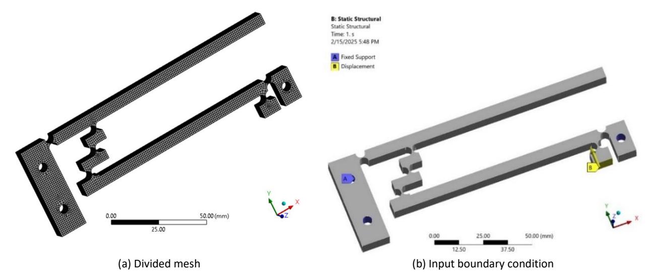
In order to analyze the stress and displacement of the amplifying compliant mechanism, the static analysis module of ANSYS software was used. First, the model was automatically meshed with a mesh size of 0.5 mm using quadrilateral elements. The resulting mesh consisted of 144,106 quadrilateral elements and 785,983 nodes, as shown in Figure 3(a). Next, boundary conditions were applied at three holes in the model using the Fixed Support tool, as indicated in blue on face A. The load was applied as an input displacement of 0.01 mm using the Displacement tool, shown in yellow in Figure 3(b). Finally, the simulation was carried out using the Solve tool, which produced the resulting displacement and stress distributions.
Divided mesh and input boundary condition for the displacement amplifier mechanism.
Multi-criteria Decision Making
Multi-criteria decision making (MCDM) plays a critical role in evaluating alternatives by enabling decision-makers to systematically consider and balance multiple, often conflicting, criteria. This approach is particularly valuable in complex scenarios where relying on a single criterion may lead to suboptimal or biased outcomes. By integrating both qualitative and quantitative factors, MCDM enhances the transparency, objectivity, and robustness of the decision-making process, ultimately leading to more informed and justifiable choices. There are many methods of decision-making. In this study, the EAMR method, SAW method, WASPAS method, and EDAS method are used. Here are the steps of the methods presented specifically as follows:
EAMR Method
EAMR is a multi-criteria decision-making method used to rank and select alternatives based on multiple criteria. It is an extended variation of the ARAS (Additive Ratio Assessment) method, which evaluates alternatives using additive ratios to compare how well each alternative matches the criteria.
Collect experimental data and arrange them into a matrix in Eq. (1):
\[X_{d} = \begin{bmatrix} x_{11} \dots x_{1n} \\ x_{21} \dots x_{2n} \\ \dots \\ x_{m1} \dots x_{mn} \end{bmatrix}\] (1)
where m is the number of experiments and n is the number of objectives.
The input data will be normalized as follows in Eq. (2)
\[n_{ij} = \frac{x_{ij}}{\max x_{ij}} \tag{2}\]
Determine the normalization matrix of weighted objectives in Eq. (3):
\[v_{ij} = w_i.n_{ij} \tag{3}\] where \(w_i\) is the weight of each objective, which is determined by the MEREC method from Eqs. (4) to (6)
\[G_i^+ = v_{i1}^+ + v_{i2}^+ + \dots + v_{im}^+\] the biggest objective is the best (4)
\[G_i^- = v_{i1}^- + v_{i2}^- + \dots + v_{im}^-\] the smallest objective is the best (5)
\[S_i = \frac{RV(G_i^+)}{RV(G_i^-)} \tag{6}\]
The optimal case is where the value of \(S_{i}\) is the largest.
SAW Method
The Simple Additive Weighting (SAW) method, also known as the simple weighted synthesis method, is a technique used to calculate the total score of each option based on the values of individual criteria and their corresponding weights. The option with the highest total score is considered the optimal choice. In this investigation, the SAW method was employed to confirm the optimal values of displacement and stress, following the approach described by (Ciardiello & Genovese, 2023; Jazaudhi'fi et al., 2024; Tafazzoli et al., 2024; Taherdoost, 2023) as follows:
Step 1: Determine the normalized values of every criterion in Eqs. (7) and (8)
\[n_{ij} = \frac{y_{ij}}{\max y_{ij}} \tag{7}\]
\[n_{ij} = \frac{\min y_{ij}}{y_{ij}} \tag{8}\]
Step 2:
\[v_i = \sum_{j=1}^{n} w_j . \, n_{ij} \tag{9}\] where \(w_i\) in Eq. (9) is the weight of each objective, which is determined by the MEREC method.
Step 3: Determine the rank of the \(v_i\). The optimal case is the case where the value of Vi is the largest.
WASPAS Method
In this investigation, the confirmation of the optimal values of displacement and stress was conducted using the WASPAS method, as proposed by (Ghorbani et al., 2025; Kavimani et al., 2024) as following:
WASPAS (Weighted Aggregated Sum Product ASsessment) is a multi-criteria decision-making (MCDM) method that combines two widely used techniques: the Weighted Sum Model (WSM) and the Weighted Product Model (WPM). This method enables the evaluation and ranking of alternatives based on multiple criteria, leveraging the strengths of both WSM and WPM to enhance the accuracy and comprehensiveness of the decision-making process in selecting the optimal solution.
Step 1: Using Eq.(7) and Eq.(8) to determine \(n_{ij}\), next to the values of \(v_{ij}\) were determined by Eq.(10), the values of \(Q_i\) were determined by Eq.(11), The values of \(P_i\) were determined by Eq. (12), and the values of \(A_i\) were determined by Eq. (13)
\[v_{ij} = w_i.n_{ij} \tag{10}\] where \(w_i\) is the weight of each objective which is determined by the MEREC method
\[Q_i = \sum_{i=1}^{n} v_{ii}\] (11)
\[P_i = \prod_{i=1}^n (v_{ii})^{w_i} \tag{12}\]
Step 2: Determine Ai
\[A_i = \lambda. Q_i + (1 - \lambda). P_i, \lambda = 0.9 \tag{13}\]
Step 3: Rank the \(A_i\) values to determine the optimal value of \(A_i\) is the largest value.
EDAS Method
EDAS (Evaluation based on Distance from Average Solution) is a method that evaluates alternatives by measuring their distance from the average solution. First, the average value for each criterion is calculated across all alternatives. Then, the distance of each alternative from this average value is determined. Finally, these distances are weighted and summed to rank the alternatives. This method is particularly useful when multiple criteria need to be considered and the optimal option must be selected based on an overall evaluation. In this investigation, the confirmation of the optimal values of displacement and stress was performed using the EDAS method, following the approaches of (Imran & Ullah, 2025; Peng et al., 2022; Ramya Sharma et al., 2024; Rasool et al., 2025; Shah & Pan, 2024; Wei et al., 2019; Wei et al., 2021; Xia, 2024; Zulgarnain et al., 2024) as described below:
Collect experimental data and arrange them into a matrix in Eq. (14):
\[X = [x_{ij}]_{m \times n} = \begin{bmatrix} x_{11} \cdots x_{1n} \\ x_{21} \cdots x_{1n} \\ \vdots \cdots x_{2n} \\ x_{m1} \cdots x_{mn} \end{bmatrix}\](14)
Determine the average value for the objectives in Eq. (15):
\[AVG = \frac{\sum_{i=1}^{m} x_i}{m} \tag{15}\]
Determine positive distance values in Eqs. (16) and (17):
\[PD_{ij} = \frac{max[0,(x_{ij}-AVG_j)]}{AVG_j}, the biggest objective is the best\] (16)
\[PD_{ij} = \frac{max[0,(AVG_j - x_{ij})]}{AVG_i}, the smallest objective is the best\] (17)
Determine negative distance values in Eqs. (18) and (19):
\[ND_{ij} = \frac{max[0,(AVG_j - x_{ij})]}{AVG_j},\] (18)
\[ND_{ij} = \frac{max[0,(x_{ij} - AVG_j)]}{AVG_i}\], the smallest objective is the best (19)
Determine the normalization matrix of weighted objectives in Eqs. (20) and (21)
\[SoP_i = \sum_{i=1}^m w_i \cdot PD_{ii} \tag{20}\]
\[SoN_i = \sum_{i=1}^m w_i \cdot ND_{ii} \tag{21}\] where \(w_i\) is the weight of each objective, which is determined by the MEREC method in Eqs. (23) to (24)
\[SSoP_i = \frac{SoP_i}{max(SoP_i)} \tag{22}\]
\[SSoN_i = \frac{SoN_i}{max(SoN_i)} \tag{23}\]
\[APS_i = \frac{1}{2}(SSoP_i + SSoN_i) \tag{24}\]
Determine the Weight
MEREC weights the impact of removing each criterion on the variability of the alternatives. The idea is that criteria that have a greater impact on the overall variability of the alternatives will be given a greater weight. This method allows for objective weighting, independent of the subjective judgment of the decision maker. The weight of each objective, which is determined by the Method based on the Removal Effects of Criteria (MEREC) method (Borchers & Pieler, 2010; Fan et al., 2024; Keshavarz-Ghorabaee, 2021; Keshavarz-Ghorabaee et al., 2021; Shanmugasundar et al., 2022) as following:
Determine the normalized values of the objective function in Eqs. (25) and (26):
\[h_{ij} = \frac{\min u_{ij}}{u_{ii}} \tag{25}\]
\[h_{ij} = \frac{u_{ij}}{\max u_{ij}} \tag{26}\]
\(u_{ij}\) are the stress and displacement values were estimated by the FEM.
Determine performance for each case in Eq. (27):
\[S_{i} = \ln \left[ 1 + \left( \frac{1}{n} \sum_{j}^{n} \left| \ln(h_{ij}) \right| \right) \right] \tag{27}\]
Determine effective performance after removing single criteria in Eq. (28)
\[S'_{ij} = \ln\left[1 + \left(\frac{1}{n}\sum_{k,k\neq j}^{n}\left|\ln\left(h_{ij}\right)\right|\right)\right] \tag{28}\]
Determine the deviation of the criteria in Eq. (28)
\[E_{j} = \left| S_{ij}^{'} - S_{i} \right| \tag{29}\]
Determine the weight for each objective in Eq. (30)
\[w_j = \frac{E_j}{\sum_k^m E_k} \tag{30}\]
Taguchi Method (TM)
To confirm the optimal results obtained from the optimization methods, the Taguchi method was utilized through signal-to-noise ratio analysis of the values Si, Vi, Ai, and APSi, applying the "larger-the-better" criterion (Abd-Elwahab et al., 2024; Georgantzinos et al., 2024; Hisam et al., 2024; Jakupi et al., 2024; Vignesh & Abdul Rahim, 2024) as follows:
\[S/N = -10\log(\frac{1}{n}\sum_{i=1}^{n}\frac{1}{v_{i}^{2}})\] (31)
\(y_i\) is the value of the i<sup>th</sup> simulation, and n is the total number of simulations
CI value was also determined at \(\alpha = 0.05\) for Si, \(V_i\), \(A_i\), and \(APS_i\) by employing Eq. (32)
\[CI_{CE} = \pm \sqrt{F_{\alpha}(1, fe)Ve(\frac{1}{n_{eff}} + \frac{1}{R_e})}\] (32)
\(F_{\alpha}(1, fe)\) value lookup in Table B-2 in reference (Roy, 2010)
Results
In this investigation, the deformation and stress of 27 models were first analyzed using the finite element method in ANSYS. These 27 models were designed with SolidWorks software based on the experimental design approach of the Taguchi method. This design approach offers the advantage of requiring fewer experiments while producing highly reliable results. Next, to select the optimal model, four multi-criteria decision-making methods were applied, and finally, the Taguchi method was used to confirm the results obtained. The finite element analysis results for stress and displacement of the 27 models were obtained through the static analysis module in ANSYS and were summarized in Table 2.
Table 3 presents the outcomes of determining weight, while Table 4 reports the results of the EAMR method. Table 5 shows the computed values of n<sub>ij</sub>, V<sub>i</sub> and rank, and the corresponding ranking of alternatives. Table 6 provides the results obtained from the WASPAS method. In Table 7, the positive distance, negative distance, SoPi, SoNi, SSoPi, SSoNi, APSi, and rank. Tables 8 and 9 summarize the signal-to-noise analysis results for S<sub>i</sub> and V<sub>i</sub>, respectively, Table 10 presents the outcomes of the signal-to-noise analysis for A<sub>i</sub>, while Table 11 shows signal-to-noise analysis for APSi.
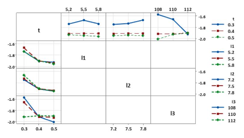
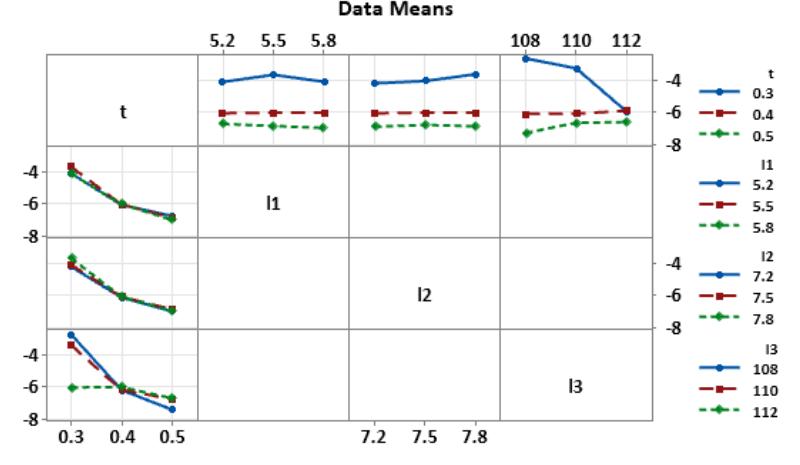
Figure 4 shows the signal-to-noise analysis graph of \(S_{i,}\) while Figure 5 and Figure 6 depict the corresponding graphs for \(V_i\) and \(A_i\), respectively. Figure 7 presents the signal-to-noise analysis graph of APSi. In addition, Figure 8, Figure 9, Figure 10, and Figure 11 display the interaction analysis outcomes for the SN of \(S_{i,}\) \(V_{i,}\) \(A_{i,}\) and APSi, respectively, providing further insight into the combined effects of the considered factors.
Table 2 The FEM results of 27 simulation cases.
| t | l1 | l2 | l3 | Di (mm) | St (MPa) |
|---|---|---|---|---|---|
| 0.3 | 5.2 | 7.2 | 108 | 0.66046 | 51.6070 |
| 0.3 | 5.2 | 7.5 | 110 | 0.67032 | 52.1470 |
| 0.3 | 5.2 | 7.8 | 112 | 0.67486 | 55.6550 |
| 0.3 | 5.5 | 7.2 | 110 | 0.67136 | 52.5000 |
| 0.3 | 5.5 | 7.5 | 112 | 0.67576 | 55.7280 |
| 0.3 | 5.5 | 7.8 | 108 | 0.65238 | 48.790 |
| 0.3 | 5.8 | 7.2 | 112 | 0.67643 | 55.7870 |
| 0.3 | 5.8 | 7.5 | 108 | 0.65364 | 50.9020 |
| 0.3 | 5.8 | 7.8 | 110 | 0.66506 | 51.9690 |
| 0.4 | 5.2 | 7.2 | 108 | 0.54453 | 47.3460 |
| 0.4 | 5.2 | 7.5 | 110 | 0.54238 | 47.1440 |
| 0.4 | 5.2 | 7.8 | 112 | 0.53570 | 46.6450 |
| 0.4 | 5.5 | 7.2 | 110 | 0.54252 | 47.1670 |
| 0.4 | 5.5 | 7.5 | 112 | 0.53562 | 46.6440 |
| 0.4 | 5.5 | 7.8 | 108 | 0.54263 | 47.1330 |
| 0.4 | 5.8 | 7.2 | 112 | 0.53542 | 46.6250 |
| 0.4 | 5.8 | 7.5 | 108 | 0.54306 | 47.1560 |
| 0.4 | 5.8 | 7.8 | 110 | 0.54274 | 47.1590 |
| 0.5 | 5.2 | 7.2 | 108 | 0.44390 | 42.9330 |
| 0.5 | 5.2 | 7.5 | 110 | 0.43447 | 41.7910 |
| 0.5 | 5.2 | 7.8 | 112 | 0.42168 | 41.1190 |
| 0.5 | 5.5 | 7.2 | 110 | 0.43408 | 41.9390 |
| 0.5 | 5.5 | 7.5 | 112 | 0.42109 | 41.1940 |
| 0.5 | 5.5 | 7.8 | 108 | 0.44596 | 43.0570 |
| 0.5 | 5.8 | 7.2 | 112 | 0.42043 | 41.3020 |
| 0.5 | 5.8 | 7.5 | 108 | 0.44585 | 43.0740 |
| 0.5 | 5.8 | 7.8 | 110 | 0.43802 | 42.2990 |
Determining Weight
Table 3 The outcomes of determining weight.
| hij | Si | Sij' | Ej | |||
|---|---|---|---|---|---|---|
| Di | St | Di | St | Di | St | |
| 0.6366 | 0.9251 | 0.2349 | 0.2036 | 0.0382 | 0.0313 | 0.1654 |
| 0.6272 | 0.9348 | 0.2366 | 0.2096 | 0.0332 | 0.0270 | 0.1765 |
| 0.6230 | 0.9976 | 0.2133 | 0.2124 | 0.0012 | 0.0010 | 0.2112 |
| 0.6262 | 0.9411 | 0.2346 | 0.2103 | 0.0299 | 0.0243 | 0.1804 |
| 0.6222 | 0.9989 | 0.2133 | 0.2129 | 0.0005 | 0.0004 | 0.2124 |
| 0.6445 | 0.8746 | 0.2521 | 0.1986 | 0.0648 | 0.0535 | 0.1337 |
| 0.6215 | 1.0000 | 0.2133 | 0.2133 | 0.0000 | 0.0000 | 0.2133 |
| 0.6432 | 0.9124 | 0.2362 | 0.1994 | 0.0448 | 0.0368 | 0.1546 |
| 0.6322 | 0.9316 | 0.2349 | 0.2064 | 0.0348 | 0.0284 | 0.1716 |
| 0.7721 | 0.8487 | 0.1917 | 0.1216 | 0.0788 | 0.0701 | 0.0428 |
| 0.7752 | 0.8451 | 0.1919 | 0.1199 | 0.0808 | 0.0720 | 0.0391 |
| 0.7848 | 0.8361 | 0.1911 | 0.1144 | 0.0857 | 0.0768 | 0.0286 |
| 0.7750 | 0.8455 | 0.1918 | 0.1200 | 0.0806 | 0.0718 | 0.0394 |
| 0.7849 | 0.8361 | 0.1911 | 0.1143 | 0.0857 | 0.0768 | 0.0286 |
| 0.7748 | 0.8449 | 0.1922 | 0.1201 | 0.0809 | 0.0721 | 0.0391 |
| 0.7852 | 0.8358 | 0.1911 | 0.1141 | 0.0859 | 0.0770 | 0.0282 |
| 0.7742 | 0.8453 | 0.1923 | 0.1204 | 0.0807 | 0.0719 | 0.0397 |
| 0.7746 | 0.8453 | 0.1920 | 0.1202 | 0.0807 | 0.0719 | 0.0395 |
| 0.9471 | 0.7696 | 0.1468 | 0.0268 | 0.1231 | 0.1200 | 0.0963 |
| 0.9677 | 0.7491 | 0.1492 | 0.0163 | 0.1349 | 0.1329 | 0.1186 |
| 0.9970 | 0.7371 | 0.1433 | 0.0015 | 0.1420 | 0.1418 | 0.1405 |
| 0.9686 | 0.7518 | 0.1472 | 0.0158 | 0.1334 | 0.1314 | 0.1175 |
| 0.9984 | 0.7384 | 0.1419 | 0.0008 | 0.1412 | 0.1411 | 0.1404 |
| 0.9428 | 0.7718 | 0.1475 | 0.0290 | 0.1218 | 0.1185 | 0.0927 |
| 1.0000 | 0.7404 | 0.1400 | 0.0000 | 0.1400 | 0.1400 | 0.1400 |
| 0.9430 | 0.7721 | 0.1473 | 0.0289 | 0.1216 | 0.1183 | 0.0927 |
| 0.9598 | 0.7582 | 0.1475 | 0.0203 | 0.1296 | 0.1272 | 0.1093 |
Results of the EAMR Method
Table 4 The outcomes of EAMR method.
| nij | vij | Gi | |||||
|---|---|---|---|---|---|---|---|
| Di | St | Di | St | Di | St | Si | Rank |
| 0.97639 | 0.92507 | 0.39515 | 0.55069 | 0.39515 | 0.55069 | 0.71755 | 4 |
| 0.99097 | 0.93475 | 0.40105 | 0.55646 | 0.40105 | 0.55646 | 0.72072 | 2 |
| 0.99768 | 0.99763 | 0.40376 | 0.59389 | 0.40376 | 0.59389 | 0.67986 | 8 |
| 0.99250 | 0.94108 | 0.40167 | 0.56022 | 0.40167 | 0.56022 | 0.71698 | 6 |
| 0.99901 | 0.99894 | 0.40430 | 0.59467 | 0.40430 | 0.59467 | 0.67988 | 7 |
| 0.96445 | 0.87459 | 0.39031 | 0.52064 | 0.39031 | 0.52064 | 0.74968 | 1 |
| 1.00000 | 1.00000 | 0.40470 | 0.59530 | 0.40470 | 0.59530 | 0.67983 | 9 |
| 0.96631 | 0.91243 | 0.39107 | 0.54317 | 0.39107 | 0.54317 | 0.71997 | 3 |
| 0.98319 | 0.93156 | 0.39790 | 0.55456 | 0.39790 | 0.55456 | 0.71751 | 5 |
| 0.80501 | 0.84869 | 0.32579 | 0.50522 | 0.32579 | 0.50522 | 0.64484 | 15 |
| 0.80183 | 0.84507 | 0.32450 | 0.50307 | 0.32450 | 0.50307 | 0.64504 | 13 |
| 0.79195 | 0.83613 | 0.32051 | 0.49774 | 0.32051 | 0.49774 | 0.64392 | 16 |
| 0.80203 | 0.84548 | 0.32459 | 0.50331 | 0.32459 | 0.50331 | 0.64490 | 14 |
| 0.79183 | 0.83611 | 0.32046 | 0.49773 | 0.32046 | 0.49773 | 0.64383 | 18 |
| 0.80220 | 0.84487 | 0.32465 | 0.50295 | 0.32465 | 0.50295 | 0.64549 | 11 |
| 0.79154 | 0.83577 | 0.32034 | 0.49753 | 0.32034 | 0.49753 | 0.64386 | 17 |
| 0.80283 | 0.84529 | 0.32491 | 0.50320 | 0.32491 | 0.50320 | 0.64569 | 10 |
| 0.80236 | 0.84534 | 0.32472 | 0.50323 | 0.32472 | 0.50323 | 0.64527 | 12 |
| 0.65624 | 0.76959 | 0.26558 | 0.45813 | 0.26558 | 0.45813 | 0.57970 | 24 |
| 0.64230 | 0.74912 | 0.25994 | 0.44595 | 0.25994 | 0.44595 | 0.58289 | 19 |
| 0.62339 | 0.73707 | 0.25229 | 0.43878 | 0.25229 | 0.43878 | 0.57498 | 25 |
| 0.64172 | 0.75177 | 0.25971 | 0.44753 | 0.25971 | 0.44753 | 0.58032 | 23 |
| 0.62252 | 0.73842 | 0.25193 | 0.43958 | 0.25193 | 0.43958 | 0.57313 | 26 |
| 0.65928 | 0.77181 | 0.26681 | 0.45946 | 0.26681 | 0.45946 | 0.58072 | 20 |
| 0.62154 | 0.74035 | 0.25154 | 0.44073 | 0.25154 | 0.44073 | 0.57074 | 27 |
| 0.65912 | 0.77212 | 0.26675 | 0.45964 | 0.26675 | 0.45964 | 0.58034 | 22 |
| 0.64755 | 0.75822 | 0.26206 | 0.45137 | 0.26206 | 0.45137 | 0.58060 | 21 |
Results of SAW Method
Table 5 The values nij, Vi and rank.
| nij | |||
|---|---|---|---|
| Di | St | Vi | Rank |
| 0.97639 | 0.79677 | 0.86946 | 4 |
| 0.99097 | 0.78852 | 0.87045 | 3 |
| 0.99768 | 0.73882 | 0.84358 | 18 |
| 0.99250 | 0.78322 | 0.86792 | 6 |
| 0.99901 | 0.73785 | 0.84354 | 20 |
| 0.96445 | 0.84276 | 0.89201 | 1 |
| 1.00000 | 0.73707 | 0.84348 | 21 |
| 0.96631 | 0.80781 | 0.87195 | 2 |
| 0.98319 | 0.79122 | 0.86891 | 5 |
| 0.80501 | 0.86848 | 0.84279 | 23 |
| 0.80183 | 0.87220 | 0.84372 | 17 |
| 0.79195 | 0.88153 | 0.84528 | 11 |
| 0.80203 | 0.87177 | 0.84355 | 19 |
| 0.79183 | 0.88155 | 0.84524 | 12 |
| 0.80220 | 0.87240 | 0.84399 | 15 |
| 0.79154 | 0.88191 | 0.84534 | 10 |
| 0.80283 | 0.87198 | 0.84399 | 14 |
| 0.80236 | 0.87192 | 0.84377 | 16 |
| 0.65624 | 0.95775 | 0.83573 | 25 |
| 0.64230 | 0.98392 | 0.84566 | 9 |
| 0.62339 | 1.00000 | 0.84759 | 7 |
| 0.64172 | 0.98045 | 0.84336 | 22 |
| 0.62252 | 0.99818 | 0.84615 | 8 |
| 0.65928 | 0.95499 | 0.83532 | 26 |
| 0.62154 | 0.99557 | 0.84420 | 13 |
| 0.65912 | 0.95461 | 0.83503 | 27 |
| 0.64755 | 0.97210 | 0.84075 | 24 |
Results WASPAS Method
Table 6 The results of the WASPAS method.
| nij | vij | ||||||
|---|---|---|---|---|---|---|---|
| Di | St | Di | St | Qi | Pi | Ai | Rank |
| 0.9764 | 0.7968 | 0.3951 | 0.4743 | 0.8695 | 0.4405 | 0.8266 | 4 |
| 0.9910 | 0.7885 | 0.4010 | 0.4694 | 0.8705 | 0.4404 | 0.8275 | 3 |
| 0.9977 | 0.7388 | 0.4038 | 0.4398 | 0.8436 | 0.4249 | 0.8017 | 18 |
| 0.9925 | 0.7832 | 0.4017 | 0.4662 | 0.8679 | 0.4389 | 0.8250 | 6 |
| 0.9990 | 0.7379 | 0.4043 | 0.4392 | 0.8435 | 0.4248 | 0.8017 | 20 |
| 0.9644 | 0.8428 | 0.3903 | 0.5017 | 0.8920 | 0.4532 | 0.8481 | 1 |
| 1.0000 | 0.7371 | 0.4047 | 0.4388 | 0.8435 | 0.4247 | 0.8016 | 21 |
| 0.9663 | 0.8078 | 0.3911 | 0.4809 | 0.8720 | 0.4423 | 0.8290 | 2 |
| 0.9832 | 0.7912 | 0.3979 | 0.4710 | 0.8689 | 0.4399 | 0.8260 | 5 |
| 0.8050 | 0.8685 | 0.3258 | 0.5170 | 0.8428 | 0.4289 | 0.8014 | 22 |
| 0.8018 | 0.8722 | 0.3245 | 0.5192 | 0.8437 | 0.4293 | 0.8023 | 16 |
| 0.7920 | 0.8815 | 0.3205 | 0.5248 | 0.8453 | 0.4298 | 0.8037 | 9 |
| 0.8020 | 0.8718 | 0.3246 | 0.5190 | 0.8436 | 0.4292 | 0.8021 | 17 |
| 0.7918 | 0.8815 | 0.3205 | 0.5248 | 0.8452 | 0.4298 | 0.8037 | 10 |
| 0.8022 | 0.8724 | 0.3247 | 0.5193 | 0.8440 | 0.4294 | 0.8025 | 14 |
| 0.7915 | 0.8819 | 0.3203 | 0.5250 | 0.8453 | 0.4299 | 0.8038 | 8 |
| 0.8028 | 0.8720 | 0.3249 | 0.5191 | 0.8440 | 0.4294 | 0.8025 | 13 |
| 0.8024 | 0.8719 | 0.3247 | 0.5191 | 0.8438 | 0.4293 | 0.8023 | 15 |
| 0.6562 | 0.9577 | 0.2656 | 0.5701 | 0.8357 | 0.4185 | 0.7940 | 25 |
| 0.6423 | 0.9839 | 0.2599 | 0.5857 | 0.8457 | 0.4216 | 0.8033 | 12 |
| 0.6234 | 1.0000 | 0.2523 | 0.5953 | 0.8476 | 0.4206 | 0.8049 | 7 |
| 0.6417 | 0.9804 | 0.2597 | 0.5837 | 0.8434 | 0.4206 | 0.8011 | 23 |
| 0.6225 | 0.9982 | 0.2519 | 0.5942 | 0.8461 | 0.4199 | 0.8035 | 11 |
| 0.6593 | 0.9550 | 0.2668 | 0.5685 | 0.8353 | 0.4186 | 0.7936 | 26 |
| 0.6215 | 0.9956 | 0.2515 | 0.5927 | 0.8442 | 0.4190 | 0.8017 | 19 |
| 0.6591 | 0.9546 | 0.2667 | 0.5683 | 0.8350 | 0.4184 | 0.7934 | 27 |
| 0.6475 | 0.9721 | 0.2621 | 0.5787 | 0.8408 | 0.4200 | 0.7987 | 24 |
Outcomes of the EDAS Method
Table 7 Positive distance, negative distance, SoPi, SoNi, SSoPi, SSoNi, APSi, and rank.
| PDij | NDij | ||||||||
|---|---|---|---|---|---|---|---|---|---|
| Di | St | Di | St | SoPi | SoNi | SSoPi | SSoNi | APSi | Rank |
| 0.20731 | 0.00000 | 0.00000 | 0.09130 | 0.08390 | 0.05435 | 0.87657 | 0.49190 | 0.68423 | 4 |
| 0.22534 | 0.00000 | 0.00000 | 0.10272 | 0.09119 | 0.06115 | 0.95277 | 0.42835 | 0.69056 | 3 |
| 0.23363 | 0.00000 | 0.00000 | 0.17690 | 0.09455 | 0.10531 | 0.98787 | 0.01553 | 0.50170 | 10 |
| 0.22724 | 0.00000 | 0.00000 | 0.11019 | 0.09196 | 0.06559 | 0.96081 | 0.38681 | 0.67381 | 6 |
| 0.23528 | 0.00000 | 0.00000 | 0.17845 | 0.09522 | 0.10623 | 0.99482 | 0.00694 | 0.50088 | 11 |
| 0.19254 | 0.00000 | 0.00000 | 0.03175 | 0.07792 | 0.01890 | 0.81411 | 0.82329 | 0.81870 | 1 |
| 0.23650 | 0.00000 | 0.00000 | 0.17969 | 0.09571 | 0.10697 | 1.00000 | 0.00000 | 0.50000 | 12 |
| 0.19485 | 0.00000 | 0.00000 | 0.07639 | 0.07885 | 0.04548 | 0.82385 | 0.57487 | 0.69936 | 2 |
| 0.21572 | 0.00000 | 0.00000 | 0.09896 | 0.08730 | 0.05891 | 0.91212 | 0.44930 | 0.68071 | 5 |
| 0.00000 | 0.00000 | 0.00461 | 0.00120 | 0.00000 | 0.00258 | 0.00000 | 0.97591 | 0.48795 | 18 |
| 0.00000 | 0.00307 | 0.00854 | 0.00000 | 0.00183 | 0.00345 | 0.01912 | 0.96770 | 0.49341 | 16 |
| 0.00000 | 0.01363 | 0.02075 | 0.00000 | 0.00811 | 0.00840 | 0.08475 | 0.92151 | 0.50313 | 8 |
| 0.00000 | 0.00259 | 0.00828 | 0.00000 | 0.00154 | 0.00335 | 0.01609 | 0.96867 | 0.49238 | 17 |
| 0.00000 | 0.01365 | 0.02089 | 0.00000 | 0.00812 | 0.00846 | 0.08488 | 0.92095 | 0.50292 | 9 |
| 0.00000 | 0.00331 | 0.00808 | 0.00000 | 0.00197 | 0.00327 | 0.02057 | 0.96943 | 0.49500 | 13 |
| 0.00000 | 0.01405 | 0.02126 | 0.00000 | 0.00836 | 0.00860 | 0.08738 | 0.91957 | 0.50347 | 7 |
| 0.00000 | 0.00282 | 0.00729 | 0.00000 | 0.00168 | 0.00295 | 0.01754 | 0.97241 | 0.49497 | 14 |
| 0.00000 | 0.00276 | 0.00788 | 0.00000 | 0.00164 | 0.00319 | 0.01715 | 0.97019 | 0.49367 | 15 |
| 0.00000 | 0.09212 | 0.18856 | 0.00000 | 0.05484 | 0.07631 | 0.57295 | 0.28664 | 0.42980 | 25 |
| 0.00000 | 0.11627 | 0.20579 | 0.00000 | 0.06922 | 0.08329 | 0.72315 | 0.22142 | 0.47229 | 19 |
| 0.00000 | 0.13048 | 0.22917 | 0.00000 | 0.07768 | 0.09275 | 0.81153 | 0.13297 | 0.47225 | 20 |
| 0.00000 | 0.11314 | 0.20651 | 0.00000 | 0.06735 | 0.08357 | 0.70368 | 0.21872 | 0.46120 | 22 |
| 0.00000 | 0.12890 | 0.23025 | 0.00000 | 0.07673 | 0.09318 | 0.80167 | 0.12889 | 0.46528 | 21 |
| 0.00000 | 0.08950 | 0.18479 | 0.00000 | 0.05328 | 0.07479 | 0.55664 | 0.30088 | 0.42876 | 26 |
| 0.00000 | 0.12661 | 0.23146 | 0.00000 | 0.07537 | 0.09367 | 0.78746 | 0.12432 | 0.45589 | 23 |
| 0.00000 | 0.08914 | 0.18499 | 0.00000 | 0.05306 | 0.07487 | 0.55441 | 0.30012 | 0.42727 | 27 |
| 0.00000 | 0.10553 | 0.19931 | 0.00000 | 0.06282 | 0.08066 | 0.65634 | 0.24597 | 0.45115 | 24 |
Confirm the Results of the Optimization Method
Table 8 Signal-to-noise analysis for Si.
| Level | t | l1 | l2 | l3 |
|---|---|---|---|---|
| 1 | -2.990 | -3.861 | -3.878 | -3.759 |
| 2 | -3.812 | -3.829 | -3.859 | -3.798 |
| 3 | -4.759 | -3.871 | -3.824 | -4.004 |
| Delta | 1.769 | 0.042 | 0.054 | 0.245 |
| Rank | 1 | 4 | 3 | 2 |
Table 9 Signal-to-noise analysis for Vi.
| Level | t | l1 | l2 | l3 |
|---|---|---|---|---|
| 1 | -1.276 | -1.419 | -1.428 | -1.391 |
| 2 | -1.471 | -1.401 | -1.417 | -1.392 |
| 3 | -1.499 | -1.427 | -1.401 | -1.464 |
| Delta | 0.222 | 0.026 | 0.028 | 0.073 |
| Rank | 1 | 4 | 3 | 2 |
Table 10 Outcomes of signal-to-noise analysis for Ai.
| Level | t | l1 | l2 | l3 |
|---|---|---|---|---|
| 1 | -1.717 | -1.861 | -1.870 | -1.831 |
| 2 | -1.909 | -1.842 | -1.859 | -1.833 |
| 3 | -1.945 | -1.868 | -1.842 | -1.907 |
| Delta | 0.229 | 0.026 | 0.028 | 0.075 |
| Rank | 1 | 4 | 3 | 2 |
Table 11 Signal-to-noise analysis for APSi.
| Level | t | l1 | l2 | l3 |
|---|---|---|---|---|
| 1 | -4.016 | -5.689 | -5.775 | -5.407 |
| 2 | -6.085 | -5.570 | -5.677 | -5.395 |
| 3 | -6.913 | -5.754 | -5.562 | -6.211 |
| Delta | 2.897 | 0.185 | 0.212 | 0.816 |
| Rank | 1 | 4 | 3 | 2 |
Signal to noise analysis graph of Si.
Signal to noise analysis graph of Vi.
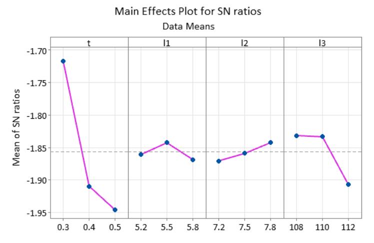
Signal to noise analysis graph of Ai.
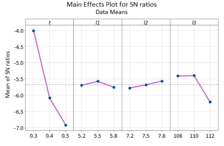
Signal to noise analysis graph of APSi.
Outcomes of Analysis Interaction
The interaction analysis outcome for SN of Si.

The interaction analysis outcome for SN of Vi.
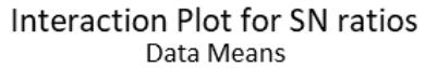
The interaction analysis outcome for SN of Ai.
The interaction analysis outcome for SN of APSi.
Table 12 Outcomes of ANOVA for Si.
| Source | DF | Seq SS | Contribution | Adj SS | Seq MS | F-Value | P-Value |
|---|---|---|---|---|---|---|---|
| t | 2 | 0.077174 | 94.13% | 0.077174 | 0.038587 | 1054.87 | 0.000 |
| l1 | 2 | 0.000061 | 0.07% | 0.000061 | 0.000031 | 0.83 | 0.455 |
| l2 | 2 | 0.000089 | 0.11% | 0.000089 | 0.000045 | 1.22 | 0.324 |
| l3 | 2 | 0.001924 | 2.35% | 0.001924 | 0.000962 | 26.29 | 0.000 |
| t*l3 | 4 | 0.002225 | 2.71% | 0.002225 | 0.000556 | 15.21 | 0.000 |
| Error | 14 | 0.000512 | 0.62% | 0.000512 | 0.000037 | ||
| Total | 26 | 0.081985 | 100.00% |
Table 13 Model summary for transformed response Si.
| S | R-sq | R-sq(adj) | PRESS | R-sq(pred) | AICc | BIC |
|---|---|---|---|---|---|---|
| 0.0060481 | 99.38% | 98.84% | 0.0019048 | 97.68% | -153.94 | -170.80 |
Table 14 Outcomes of ANOVA for Vi.
| Source | DF | Seq SS | Contribution | Adj SS | Seq MS | F-Value | P-Value |
|---|---|---|---|---|---|---|---|
| t | 2 | 0.002583 | 51.62% | 0.002583 | 0.001291 | 69.86 | 0.000 |
| l1 | 2 | 0.000033 | 0.66% | 0.000033 | 0.000016 | 0.89 | 0.432 |
| l2 | 2 | 0.000036 | 0.73% | 0.000036 | 0.000018 | 0.98 | 0.399 |
| l3 | 2 | 0.000311 | 6.22% | 0.000311 | 0.000156 | 8.42 | 0.004 |
| t*l3 | 4 | 0.001781 | 35.60% | 0.001781 | 0.000445 | 24.09 | 0.000 |
| Error | 14 | 0.000259 | 5.17% | 0.000259 | 0.000018 | ||
| Total | 26 | 0.005002 | 100.00% |
Table 15 Model Summary for Transformed Response Vi.
| S | R-sq | R-sq(adj) | PRESS | R-sq(pred) | AICc | BIC |
|---|---|---|---|---|---|---|
| 0.0042993 | 94.83% | 90.39% | 0.0009625 | 80.76% | -172.37 | -189.23 |
Table 16 Outcomes of ANOVA for Ai.
| Source | DF | Seq SS | Contribution | Adj SS | Seq MS | F-Value | P-Value |
|---|---|---|---|---|---|---|---|
| t | 2 | 0.002396 | 52.03% | 0.002396 | 0.001198 | 71.30 | 0.000 |
| l1 | 2 | 0.000029 | 0.64% | 0.000029 | 0.000015 | 0.87 | 0.440 |
| l2 | 2 | 0.000033 | 0.72% | 0.000033 | 0.000016 | 0.98 | 0.399 |
| l3 | 2 | 0.000298 | 6.47% | 0.000298 | 0.000149 | 8.87 | 0.003 |
| t*l3 | 4 | 0.001614 | 35.04% | 0.001614 | 0.000403 | 24.01 | 0.000 |
| Error | 14 | 0.000235 | 5.11% | 0.000235 | 0.000017 | ||
| Total | 26 | 0.004605 | 100.00% |
Table 17 Model summary for transformed response Ai.
| S | R-sq | R-sq(adj) | PRESS | R-sq(pred) | AICc | BIC |
|---|---|---|---|---|---|---|
| 0.0040992 | 94.89% | 90.51% | 0.0008750 | 81.00% | -174.95 | -191.81 |
Table 18 Outcomes of ANOVA for APSi.
| Source | DF | Seq SS | Contribution | Adj SS | Seq MS | F-Value | P-Value |
|---|---|---|---|---|---|---|---|
| t | 2 | 0.172275 | 62.40% | 0.172275 | 0.086138 | 135.12 | 0.000 |
| l1 | 2 | 0.001078 | 0.39% | 0.001078 | 0.000539 | 0.85 | 0.450 |
| l2 | 2 | 0.001387 | 0.50% | 0.001387 | 0.000694 | 1.09 | 0.364 |
| l3 | 2 | 0.021151 | 7.66% | 0.021151 | 0.010576 | 16.59 | 0.000 |
| t*l3 | 4 | 0.071286 | 25.82% | 0.071286 | 0.017821 | 27.96 | 0.000 |
| Error | 14 | 0.008925 | 3.23% | 0.008925 | 0.000637 | ||
| Total | 26 | 0.276103 | 100.00% |
Table 19 Model summary for transformed response APSi.
| S | R-sq | R-sq(adj) | PRESS | R-sq(pred) | AICc | BIC |
|---|---|---|---|---|---|---|
| 0.0252481 | 96.77% | 94.00% | 0.0331938 | 87.98% | -76.78 | -93.63 |
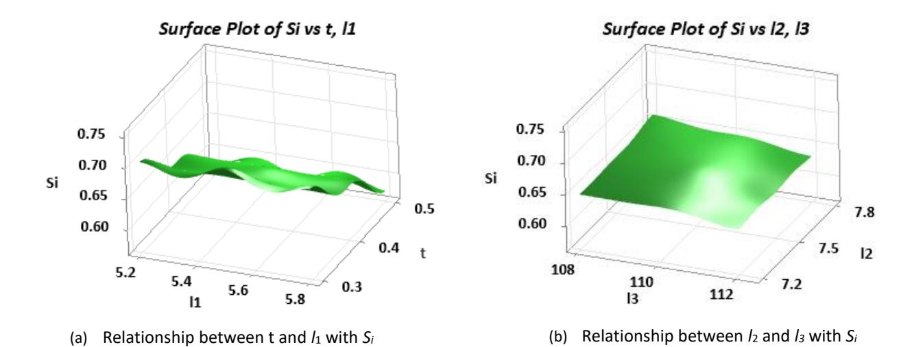
The 3D surface graph showing the relationship between design variables and Si.
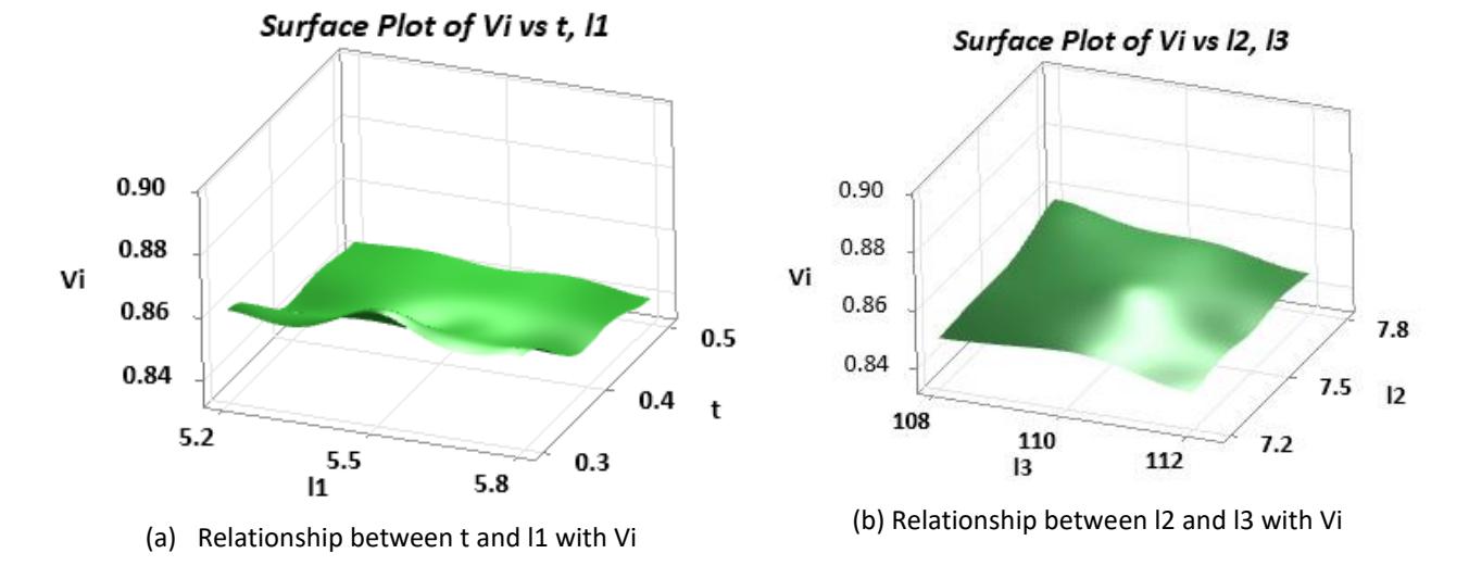
The 3D surface graph showing the relationship between design variables and Vi.
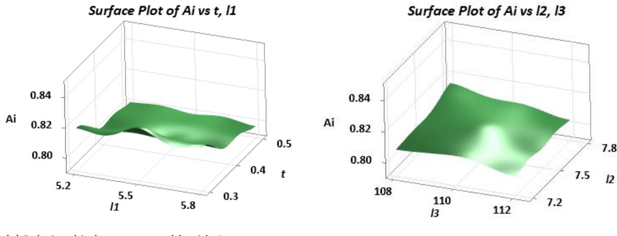
(a) Relationship between t and l1 with Ai
(b) Relationship between l2 and l3 with Ai
3D surface graph showing the relationship between design variables and Vi.
3D surface graph showing the relationship between design variables and Vi.
The predicted values of Si, Vi, Ai, and APSi obtained by the Taguchi method of Minitab software, as illustrate in Table 21 and Table 22 in row 6, are 0.742046, 0.88684, 0.8432, and 0.7978, respectively.
At 95% confidence interval, the CI values for Si, Vi, Ai, and ASPi were found to be ±0.0007832, ±009043, ±0.00798, and 0.02153, respectively, by Equation (35) as following:
For Si:
\[CI_{CE} = \pm \sqrt{4.6001 \times 0.000009 \times (\frac{1}{\frac{27}{1+12}} + 1)} = \pm 0.007832 \ 0.734214 < \mu_{confirmation} < 0.749878\] where, α = 0.05, fe = 14, F0.05(1,14) = 4.6001 [45], Ve = 0.000009, R = 12, Re = 1, n = 27.
For Vi
\[CI_{CE} = \pm \sqrt{4.6001 \times 0.000012 \times (\frac{1}{27} + 1)} = \pm 0.009043 \ 0.877797 < \mu_{confirmation} < 0.895883\] where, α = 0.05, fe = 14, F0.05(1,14) = 4.6001 [45], Ve = 0.000012, R = 12, Re = 1, n = 27.
For Ai:
\[CI_{CE} = \pm \sqrt{4.6001 \times 0.000011 \times (\frac{1}{\frac{27}{1+12}} + 1)} = \pm 0.007983 \ 0.83454 < \mu_{confirmation} < 0.85186\] where, α = 0.05, fe = 14, F0.05(1,14) = 4.6001(Roy, 2010), Ve = 0.000011, R = 12, Re = 1, n = 27.
For APSi:
\[CI_{CE} = \pm \sqrt{4.6001 \times 0.00008 \times (\frac{1}{\frac{27}{1+12}} + 1)} = \pm 0.02153 \ 0.77445 < \mu_{confirmation} < 0.82115\] where, α = 0.05, fe = 14, F0.05(1,14) = 4.6001(Roy, 2010), Ve = 0.00008, R = 12, Re = 1, n = 27.
The optimum displacement and stress results obtained are 0.65327 mm and 48.795 MPa, respectively, as depicted in Figures 16(a) and 16(b).
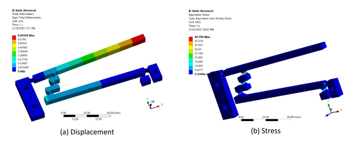
Optimal results of displacement and stress.
Discussions
The stress and displacement values summarized in Table 2. varied across the 27 cases, indicating that the design dimensions significantly affected the stress and displacement of the proposed compliant mechanism.
The weights are determined by the MEREC method, and the results are archived by inputting the Di and St values into Eq. (25) and Eq. (26), as shown in Table 3. The second and third columns were the results of Eq.(25) and Eq. (26). The fourth column was the results of Eq.(27). The fifth and sixth columns were the results of Eq. (28). The seventh and eighth columns were the results of Eq. (29). The weight of displacement and stress were obtained 0.4047 0.4047 and 0.5953, respectively by Eq. (30).
The outcomes of the EAMR method were archived by inputting the Di and St values into Eq. (2), as listed in Table 4. The second and third columns were the results of Eq. (2). The fourth and fifth columns were the results of Eq. (3). The sixth and seventh columns were the results of Eq. (4) and Eq.(5). The eighth column was the results of Eq. (6). The 9th column is the Si ranking column. The largest Si value is ranked 1st and continues to rank until the smallest Si value is ranked 27th . As presented in this Table, the sixth case with the largest Si value is ranked 1st as the optimal case. The optimal model obtained has the size of variable t as 0.3 mm, variable l1 as 5.5 mm, variable l2 as 7.8 mm, and variable l3 as 108 mm. The optimum value of Si obtained is 0.74968. The model's optimum displacement and optimum stress are obtained as 0.65238 mm and 48.790 MPa, respectively. 27 Si values are completely different, which proves that the design dimensions strongly affect the Di and St of the amplifier-compliant mechanism model flexure hinge.
The outcomes of the SAW method were archived by inputting the Di and St values into Eq. (7) and Eq. (8), as listed in Table 5. The second and third columns were the results of Eq. (7) and Eq. (8). The fourth column was the results of Eq. (9). The fifth column is the Vi ranking column. The largest Vi value is ranked 1st and continues to rank until the smallest Vi value is ranked 27th. As presented in this Table, the sixth case with the largest Vi value is ranked 1st as the optimal case. The optimal model obtained has the size of variable t as 0.3 mm, variable l1 as 5.5 mm, variable l2 as 7.8 mm, and variable l3 as 108 mm. The optimum value of Vi obtained is 0.89201. The model's optimum displacement and optimum
stress are obtained as 0.65238 mm and 48.790 MPa, respectively. 27 Vi values are completely different, which proved that the designed dimensions strongly affect the Di and St of the amplifier-compliant mechanism model flexure hinge. These results were consistent with the results of the finite element analysis method and the EAMR method.
The outcomes of the WASPAS method were archived by inputting the Di and St values into Eq.(14) and Eq.(8), as listed in Table 6. The second and third columns were the results of Eq.(16) and Eq.(17). The fourth and fifth columns were the results of Eq. (10). The sixth column was the results of Eq.11). The seventh column was the results of Eq. (12). The eighth column was the values Ai which were determined by Eq. (13). The ninth was ranking column of Ai. The largest Ai value is ranked 1st and continues to rank until the smallest Ai value is ranked 27th. As presented in this Table, the sixth case with the largest Si value is ranked 1st as the optimal case. The optimal model obtained has the size of variable t as 0.3 mm, variable l1 as 5.5 mm, variable l2 as 7.8 mm, and variable l3 as 108 mm. The optimum value of Ai obtained is 0.8481. The model's optimum Di and optimum St are obtained as 0.65238 mm and 48.790 MPa, respectively. 27 Si values are completely different, which proves that the designed dimensions strongly affect the Di and St of the amplifier-compliant mechanism model flexure hinge. These results were consistent with the results of the finite element analysis method, the results of the EAMR method, and the results of the SAW method.
The results of the EDAS method were archived by inputting the Di and St values into Eq. (14), as listed in Table 7. The second and third columns were the results of Eq. (16) and Eq.(17). The fourth and fifth columns were the results of Eq.(18) and Eq.(19). The sixth column was the results of Eq.(20). The seventh column was the results of Eq.(21). The eighth column was the results of Eq. (22). The ninth was the results of Eq. (23). The tenth column was the results of Eq. (24). The eleventh column ranking column of APSi. The largest APSi value is ranked 1st and continues to rank until the smallest APSi value is ranked 27th. As presented in this Table, the sixth case with the largest Si value is ranked 1st as the optimal case. The optimal model obtained has the size of variable t as 0.3 mm, variable l1 as 5.5 mm, variable l2 as 7.8 mm, and variable l3 as 108 mm. The optimum value of Si obtained is 0.8187. The optimum displacement and optimum stress of the model are obtained as 0.65238 mm and 48.790 MPa, respectively. 27 APSi values are completely different, which proved that the designed dimensions strongly affect the Di and St of the amplifier-compliant mechanism model flexure hinge. These results were consistent with the results of the finite element analysis method, the EAMR method, the SAW method, the SAW method and the WASPAS method.
To confirm the reliability of the EAMR method, Taguchi analysis method is applied. The Taguchi analysis results for the EAMR method are shown in Table 8. In this table it is shown that variable t affects Si the most or displacement and stress because the deviation of the mean value of Si is the largest 1.769, followed by variable l3. Next is variable l2 and finally variable l1.
The values in Table 8 were utilized to draw the graph, as presented in Figure 4. which indicated that variable t has the most influence because the slope of the graph is the largest, followed by variable l3. Next is variable l2, and finally, variable l1. This is consistent with the results of finite element analysis and the optimal result obtained is the 6th case consistent with the optimal result of the EAMR method. Accordingly, the variable t reaches its optimal value at level 1 of 0.3 mm, the variable l1 reaches its optimal value at level 2 of 5.5 mm, the variable l2 reaches its optimal value at level 3 of 7.8 mm, and the variable l3 reaches its optimal value at level 1 of 108 mm.
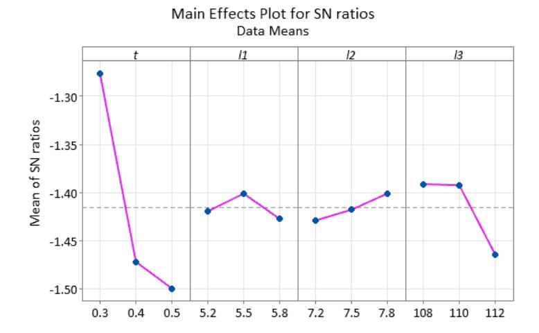
Similarly, to confirm the reliability of the SAW method, Taguchi analysis method is applied. The Taguchi analysis results for the SAW method are shown in Table 9. In this table it is shown that variable t affects Vi the most or displacement and stress because the deviation of the mean value of Vi is the largest 0.222; next is variable l3. Next is variable l2 and finally variable l1.
The values in Table 9 were utilized to draw the graph, as depicted in Figure 5 which indicated that variable t has the most influence because the slope of the graph is the largest, followed by variable l3. Next is variable l2, and finally, variable l1. This is consistent with the results of finite element analysis, and the optimal result obtained is the 6th case, which is consistent with the optimal result of the SAW method. Accordingly, the variable t reaches its optimal value at level 1 of 0.3 mm, the variable l1 reaches its optimal value at level 2 of 5.5 mm, the variable l2 reaches its optimal value at level 3 of 7.8 mm, and the variable l3 reaches its optimal value at level 1 of 108 mm. These results are consistent with the EAMR method.
Similarly, the Taguchi analysis method is applied to confirm the reliability of the WASPAS method. The Taguchi analysis results for the WASPAS method are shown in Table 10. In this table, it is shown that variable t affects Ai the most or displacement and stress because the deviation of the mean value of Vi is the largest 0.229, followed by variable l3. Next is variable l2 and finally variable l1.
The values in Table 10 were utilized to draw the graph, as illustrated in Figure 6 which pointed out that variable t has the most influence because the slope of the graph is the largest. In this figure, it is also indicated that variable t has the most influence because the slope of the graph is the largest, followed by variable l3. Next is variable l2, and finally, variable l1. This is consistent with the results of finite element analysis and the optimal result obtained is the 6th case consistent with the optimal result of the SAW method. Accordingly, the variable t reaches its optimal value at level 1 of 0.3 mm, the variable l1 reaches its optimal value at level 2 of 5.5 mm, the variable l2 reaches its optimal value at level 3 of 7.8 mm, and the variable l3 reaches its optimal value at level 1 of 108 mm. These results are consistent with the EAMR method and the SAW method.
Similarly, to verify the reliability of the EDAS method, the Taguchi analysis is applied. The Taguchi analysis results for the EDAS method are shown in Table 11. This Table, indicated that variable t affects APSi the most or displacement and stress because the deviation of the mean value of Vi is the largest 0.229, followed by variable l3. Next is variable l2 and finally variable l1.
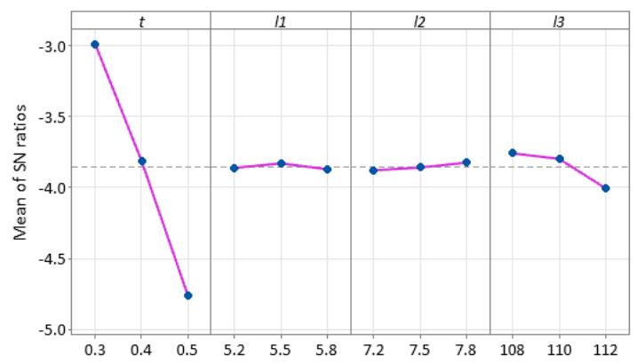
The values in Table 11 were utilized to draw the graph, as demonstrated in Figure 7 which proved that variable t has the most influence because the slope of the graph is the largest, followed by variable l3. Next is variable l2, and finally, variable l1. This is consistent with the results of finite element analysis, and the optimal result obtained is the 6th case, which is consistent with the optimal result of the EDAS method. Accordingly, the variable t reaches its optimal value at level 1 of 0.3 mm, the variable l1 reaches its optimal value at level 2 of 5.5 mm, the variable l2 reaches its optimal value at level 3 of 7.8 mm, and the variable l3 reaches its optimal value at level 1 of 108 mm. These results are consistent with the EAMR method and the SAW method.
The results of the SN interaction analysis of Si, presented in Figure 8, pointed out that the designed dimensions strongly affected Di and St. Since the lines of the graph are not parallel to each other, this proves that the selected design variables are appropriate, and the results are also consistent with those of the finite element analysis.
The results of the SN interaction analysis of Vi, presented in Figure 9, indicated that the design variables strongly affect displacement and stress. Since the lines of the graph are not parallel to each other, these proved that the selected design variables are appropriate, and the results are also consistent with the outcomes of the FEM. The results of the SN interaction analysis of Ai, presented in Figure 10, indicated that the design variables strongly affect displacement and stress. Since the lines of the graph are not parallel to each other, these proved that the selected design variables are appropriate, and the results are also consistent with the outcomes of the FEM.
The results of the SN interaction analysis of APSi, as presented in Figure 11 which indicated that the design variables strongly affect displacement and stress. Since the lines of the graph are not parallel to each other, these proved that the selected design variables are appropriate, and the results are also consistent with the outcomes of the FEM.
Results of Analysis of Variance (ANOVA)
In addition, to confirm the reliability of the FEM results and the optimum results of the EAMR method. Variance analysis is also used to do this, and the results obtained are listed in Table 12. In this Table, it is also shown that variable t has the most influence because the slope of the graph is the largest, followed by variable l3. Next is variable l2, and finally, variable l1. Because the percentage contributions of variables t, l3, l2, and l1 are 94.13%, 0.07%, 0.11%, and 2.35%, respectively. The variables t and l3 strongly influence the displacement and stress or strongly influence the Si values. Because the P values all satisfy the condition of being less than 0.05, and the F values all satisfy the condition of being greater than 2. While the variables l2 and l3 has little effected on displacement and stress of the structure because Pvalues are greater than 0.05 and F-values are less than 2. The analysis of variance results indicated that the FEM results and the optimization results of the EAMR method are reliable and in good agreement. Because variable t has the most influence because the slope of the graph is the largest, followed by variable l3. Next is variable l2 and finally variable l1, and all the R-square values are above 99%, as noted in Table 13.
In addition, to determine the reliability of the FEM results and the results of the SAW optimization method. Variance analysis was also used to do this, and the results obtained are listed in Table 14. In this Table, it was also shown that variable t has the most influence because the slope of the graph is the largest, followed by variable l3. Next is variable l2, and finally, variable l1. Because the percentage contributions of variables t, l3, l2, and l1 are 51.62%, 0.66%, 0.73%, and 6.22%, respectively. The variables t and l3 strongly influence the displacement and stress or strongly influence the Si values. Because the P values all satisfy the condition of being less than 0.05, and the F values all satisfy the condition of being greater than 2. While the variables l2 and l3 has little effected on displacement and stress of the structure because P-values are greater than 0.05 and F-values are less than 2. The analysis of variance results indicated that the FEM results and the optimization results of the SAW method are reliable and in good agreement. Because variable t has the most influence because the slope of the graph is the largest, followed by variable l3. Next is variable l2 and finally variable l1, and all the R-square values are above 94%, as noted in Table 15.
In addition, to determine the reliability of the FEM results and the results of the WASPAS optimization method. Variance analysis was also used to do this, and the results obtained are listed in Table 16. In this Table, it was also shown that variable t has the most influence because the slope of the graph is the largest, followed by variable l3. Next is variable l2, and finally, variable l1. Because the percentage contributions of variables t, l3, l2, and l1 are 52.3%, 0.64%, 0.72%, and 6.47%, respectively. The variables t and l3 strongly influence the displacement and stress or strongly influence the Si values. Because the P values all satisfy the condition of being less than 0.05, and the F values all satisfy the condition of being greater than 2. While the variables l2 and l3 has little effected on displacement and stress of the structure because P-values are greater than 0.05 and F-values are less than 2. The analysis of variance results indicated that the FEM results and the optimization results of the WASPAS method are reliable and in good agreement. Because variable t has the most influence because the slope of the graph is the largest, followed by variable l3. Next is variable l2 and finally, variable l1, and all the R-square values are above 94%, as noted in Table 17.
In addition, to determine the reliability of the FEM results and the results of the EDAS optimization method. Variance analysis is also used to do this, and the results obtained are listed in Table 18. In this Table, it was also shown that variable t has the most influence because the slope of the graph is the largest, followed by variable l3. Next is variable l2, and finally, variable l1. Because the percentage contributions of variables t, l3, l2, and l1 are 62.4%, 0.39%, 0.5%, and 7.66%, respectively. The variables t and l3 strongly influence the displacement and stress or strongly influence the Si values. Because the P values all satisfy the condition of being less than 0.05, and the F values all satisfy the condition of being greater than 2. While the variables l2 and l3 has little effected on displacement and stress of the structure because P-values are greater than 0.05 and F-values are less than 2. The analysis of variance results indicated that the FEM results and the optimization results of the EDAS method are reliable and in good agreement. Because variable t has the most influence because the slope of the graph is the largest, followed by variable l3. Next is variable l2 and finally variable l1, and all the R-square values are above 96%, as noted in Table 19.
Results Analysis of the 3D Surface Plot
Observing the graph presented in Figure 12a indicated that variable t affected the Si value more than variable l1 because when variable t changed from 0.3 mm to 0.5 mm, the Si values changed from 0.6 to greater than 0.7. When l1 increased from 5.2 mm to 5.8 mm, the Si values changed insignificantly. Figure 12b shows that variable l3 affected the Si value more than variable l2. Because when variable l3 increased from 108 mm to 112 mm, the Si value increased from 0.6 to 0.7. While the value l2 increased from 7.2 mm to 7.3 mm, the Si value changed little. These things proved that the results of 3D surface graph analysis for the EAMR method were consistent with those of the finite element, Taguchi, and variance analyses. Because variable t has the most influence because the slope of the graph is the largest, followed by variable l3. Next is variable l2, and finally, variable l1.
Observing the graph presented in Figure 13a indicated that variable t affected the Vi value more than variable l1 because when variable t changed from 0.3 mm to 0.5 mm, the Vi values changed from 0.84 to greater than 0.86. The Vi values changed insignificantly when l1 increased from 5.2 mm to 5.8 mm. Figure 13b pointed out that variable l3 affected the Vi value more than variable l2. When variable l3 increases from 108 mm to 112 mm, Vi value increases from 0.84 to 0.86. While the value l2 increased from 7.2 mm to 7.8 mm, the Vi value changed little. These things proved that the results of 3D surface graph analysis for the SAW method were consistent with those of the finite element, the Taguchi, and variance analyses. Because variable t has the most influence because the slope of the graph is the largest, followed by variable l3. Next is variable l2, and finally, variable l1.
Observing the graph presented in Figure 14a indicated that variable t affected the Ai value more than variable l1 because when variable t changed from 0.3 mm to 0.5 mm, the Ai values changed from 0.80 to greater than 0.82. The Ai values changed insignificantly when l1 increased from 5.2 mm to 5.8 mm. Figure 14b pointed out that variable l3 affected the Ai value more than variable l2. Because when variable l3 increases from 108 mm to 112 mm, the Ai value increases from 0.80 to 0.81. While the value I2 increased from 7.2 mm to 7.8 mm, the Ai value changed little. These things proved that the results of 3D surface graph analysis for the WASPAS method were consistent with those of the finite element, Taguchi, and variance analyses. Because variable t has the most influence because the slope of the graph is the largest, followed by variable \(I_3\). Next is variable \(I_2\), and finally, variable \(I_3\).
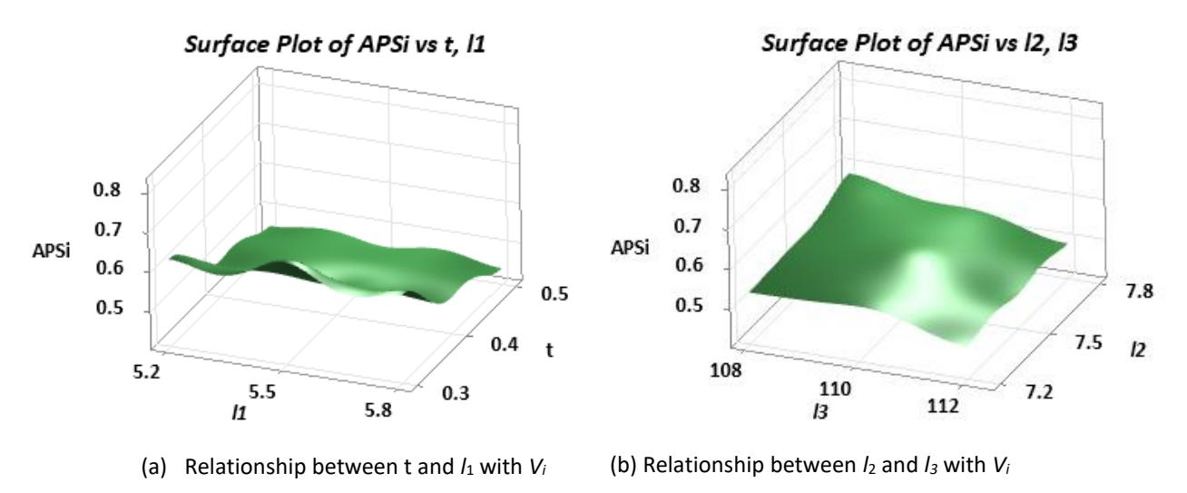
Observing the graph presented in Figure 15a indicated that variable t affected the APS<sub>i</sub> value more than variable \(l_1\) because when variable t changed from 0.3 mm to 0.5 mm, the APS<sub>i</sub> values changed from 0.50 to greater than 0.6. When \(l_2\) increased from 5.2 mm to 5.8 mm, the APSi values changed insignificantly. Figure 15b shows that variable \(l_3\) affected the APS<sub>i</sub> value more than variable \(l_2\). Because when variable \(l_3\) increases from 108 mm to 112 mm, the APS<sub>i</sub> value increases from 0.5 to 0.6. While the value \(l_2\) increased from 7.2 mm to 7.8 mm, the APS<sub>i</sub> value changed little. These things proved that the results of 3D surface graph analysis for the EDAS method were consistent with those of the finite element, Taguchi, and variance analyses. Because variable t has the most influence because the slope of the graph is the largest, followed by variable \(l_3\). Next is variable \(l_2\), and finally, variable \(l_3\).
The predicted Di and ST values of the Taguchi method are close to the \(D_i\) and ST values obtained by finite element analysis, as shown in Table 20. The error between the predicted values and the values obtained by FEM of Di is not more than 0.1%. The error between the predicted values and the values obtained by FEM of ST is not more than 1.1%. This proved that the results obtained are very reliable.
Table 20 Comparison of finite element analysis results and prediction results of the Taguchi method for Di and ST.
| Di | ST | |||||
|---|---|---|---|---|---|---|
| FEM result | Predicted result | Error (%) | FEM result | Predicted result | Error (%) | |
| 0.66046 | 0.66006 | 0.06 | 51.607 | 51.29344 | 0.61 | |
| 0.67032 | 0.67064 | 0.05 | 52.147 | 52.69178 | 1.03 | |
| 0.67486 | 0.67494 | 0.01 | 55.655 | 55.42378 | 0.42 | |
| 0.67136 | 0.67144 | 0.01 | 52.5 | 52.26878 | 0.44 | |
| 0.67576 | 0.67536 | 0.06 | 55.728 | 55.41444 | 0.57 | |
| 0.65237 | 0.65269 | 0.05 | 48.795 | 49.33978 | 1.10 | |
| 0.67643 | 0.67675 | 0.05 | 55.787 | 56.33178 | 0.97 | |
| 0.65364 | 0.65372 | 0.01 | 50.902 | 50.67078 | 0.46 | |
| 0.66506 | 0.66466 | 0.06 | 51.969 | 51.65544 | 0.61 | |
| 0.54453 | 0.54408 | 0.08 | 47.346 | 47.29844 | 0.10 | |
| 0.54238 | 0.54275 | 0.07 | 47.144 | 47.17878 | 0.07 | |
| 0.5357 | 0.53578 | 0.02 | 46.645 | 46.65778 | 0.03 | |
| 0.54252 | 0.54260 | 0.02 | 47.167 | 47.17978 | 0.03 | |
| 0.53562 | 0.53517 | 0.08 | 46.644 | 46.59644 | 0.10 | |
| 0.54263 | 0.54300 | 0.07 | 47.133 | 47.16778 | 0.07 | |
| 0.53542 | 0.53579 | 0.07 | 46.625 | 46.65978 | 0.07 | |
| 0.54306 | 0.54314 | 0.02 | 47.156 | 47.16878 | 0.03 | |
| 0.54274 | 0.54229 | 0.08 | 47.159 | 47.11144 | 0.10 | |
| 0.4439 | 0.44351 | 0.09 | 42.933 | 42.86967 | 0.15 | |
| 0.43447 | 0.43479 | 0.07 | 41.791 | 41.81967 | 0.07 | |
| 0.42168 | 0.42175 | 0.02 | 41.119 | 41.15367 | 0.08 | |
| 0.43408 | 0.43415 | 0.02 | 41.939 | 41.97367 | 0.08 | |
| 0.42109 | 0.42070 | 0.09 | 41.194 | 41.13067 | 0.15 | |
| 0.44596 | 0.44628 | 0.07 | 43.057 | 43.08567 | 0.07 | |
| 0.42043 | 0.42075 | 0.08 | 41.302 | 41.33067 | 0.07 | |
| 0.44585 | 0.44592 | 0.02 | 43.074 | 43.10867 | 0.08 | |
| 0.43802 | 0.43763 | 0.09 | 42.299 | 42.23567 | 0.15 | |
The predicted Si and Vi values of the Taguchi method are close to the Si and Vi values obtained by finite element analysis, as shown in Table 21. The error between the predicted values and the values obtained by FEM of Si is not more than 1.2%. The error between the predicted values and the values obtained by FEM of Vi is not more than 0.7%. This proved that the results obtained are very reliable.
The predicted \(A_i\) and APS<sub>i</sub> values of the Taguchi method are closed to the \(A_i\) and APS<sub>i</sub> values obtained by FEM, as shown in Table 22. The error between the predicted values and the values obtained by FEM of \(A_i\) is not more than 0.7%. The error between the predicted values and the values obtained by FEM of APS<sub>i</sub> is not more than 7%. This proved that the results obtained are very reliable.
Table 21 Comparison of finite element analysis results and prediction results of the Taguchi method for \(S_i\) and \(V_i\).
| Si | Vi | ||||
|---|---|---|---|---|---|
| FEM result | Predicted result | Error (%) | FEM result | Predicted result | Error (%) |
| 0.71755 | 0.72168 | 0.57 | 0.86946 | 0.87230 | 0.33 |
| 0.72072 | 0.71309 | 1.07 | 0.87045 | 0.86528 | 0.60 |
| 0.67986 | 0.68337 | 0.51 | 0.84358 | 0.84591 | 0.28 |
| 0.71698 | 0.72049 | 0.49 | 0.86792 | 0.87025 | 0.27 |
| 0.67988 | 0.68401 | 0.60 | 0.84354 | 0.84638 | 0.34 |
| 0.74968 | 0.74205 | 1.03 | 0.89201 | 0.88684 | 0.58 |
| 0.67983 | 0.67220 | 1.14 | 0.84348 | 0.83831 | 0.62 |
| 0.71997 | 0.72348 | 0.48 | 0.87195 | 0.87428 | 0.27 |
| 0.71751 | 0.72164 | 0.57 | 0.86891 | 0.87175 | 0.33 |
| 0.64484 | 0.64495 | 0.02 | 0.84279 | 0.84304 | 0.03 |
| 0.64504 | 0.64500 | 0.01 | 0.84372 | 0.84356 | 0.02 |
| 0.64392 | 0.64384 | 0.01 | 0.84528 | 0.84519 | 0.01 |
| 0.64490 | 0.64482 | 0.01 | 0.84355 | 0.84346 | 0.01 |
| 0.64383 | 0.64394 | 0.02 | 0.84524 | 0.84549 | 0.03 |
| 0.64549 | 0.64545 | 0.01 | 0.84399 | 0.84383 | 0.02 |
| 0.64386 | 0.64382 | 0.01 | 0.84534 | 0.84518 | 0.02 |
| 0.64569 | 0.64561 | 0.01 | 0.84399 | 0.84390 | 0.01 |
| 0.64527 | 0.64538 | 0.02 | 0.84377 | 0.84402 | 0.03 |
| 0.57970 | 0.58005 | 0.06 | 0.83573 | 0.83639 | 0.08 |
| 0.58289 | 0.58293 | 0.01 | 0.84566 | 0.84547 | 0.02 |
| 0.57498 | 0.57459 | 0.07 | 0.84759 | 0.84713 | 0.05 |
| 0.58032 | 0.57993 | 0.07 | 0.84336 | 0.84290 | 0.05 |
| 0.57313 | 0.57348 | 0.06 | 0.84615 | 0.84681 | 0.08 |
| 0.58072 | 0.58076 | 0.01 | 0.83532 | 0.83513 | 0.02 |
| 0.57074 | 0.57078 | 0.01 | 0.84420 | 0.84401 | 0.02 |
| 0.58034 | 0.57995 | 0.07 | 0.83503 | 0.83457 | 0.06 |
| 0.58060 | 0.58095 | 0.06 | 0.84075 | 0.84141 | 0.08 |
Table 22 Comparison of finite element analysis results and prediction results of the Taguchi method for \(A_i\) and APS<sub>i</sub>.
| - | Ai | APSi | |||
|---|---|---|---|---|---|
| Predicted | Error | FEM | Predicted | Error | |
| FEM result | result | (%) | result | result | (%) |
| 0.82660 | 0.82930 | 0.33 | 0.68423 | 0.70117 | 2.42 |
| 0.82750 | 0.82257 | 0.60 | 0.69056 | 0.65969 | 4.68 |
| 0.80170 | 0.80393 | 0.28 | 0.50170 | 0.51563 | 2.70 |
| 0.82500 | 0.82723 | 0.27 | 0.67381 | 0.68774 | 2.02 |
| 0.80170 | 0.80440 | 0.34 | 0.50088 | 0.51782 | 3.27 |
| 0.84810 | 0.84317 | 0.59 | 0.81870 | 0.79783 | 2.62 |
| 0.80160 | 0.79667 | 0.62 | 0.50000 | 0.46913 | 6.58 |
| 0.82900 | 0.83123 | 0.27 | 0.69936 | 0.71329 | 1.95 |
| 0.82600 | 0.82870 | 0.33 | 0.68071 | 0.69765 | 2.43 |
| 0.80140 | 0.80163 | 0.03 | 0.48795 | 0.48943 | 0.30 |
| 0.80230 | 0.80213 | 0.02 | 0.49341 | 0.49244 | 0.20 |
| 0.80370 | 0.80363 | 0.01 | 0.50313 | 0.50263 | 0.10 |
| 0.80210 | 0.80203 | 0.01 | 0.49238 | 0.49188 | 0.10 |
| 0.80370 | 0.80393 | 0.03 | 0.50292 | 0.50440 | 0.29 |
| 0.80250 | 0.80233 | 0.02 | 0.49500 | 0.49403 | 0.20 |
| 0.80380 | 0.80363 | 0.02 | 0.50347 | 0.50250 | 0.19 |
| 0.80250 | 0.80243 | 0.01 | 0.49497 | 0.49447 | 0.10 |
| 0.80230 | 0.80253 | 0.03 | 0.49367 | 0.49515 | 0.30 |
| 0.79400 | 0.79462 | 0.08 | 0.42980 | 0.43260 | 0.65 |
| 0.80330 | 0.80312 | 0.02 | 0.47229 | 0.47152 | 0.16 |
| 0.80490 | 0.80446 | 0.06 | 0.47225 | 0.47022 | 0.43 |
| 0.80110 | 0.80066 | 0.06 | 0.46120 | 0.45917 | 0.44 |
| 0.80350 | 0.80412 | 0.08 | 0.46528 | 0.46808 | 0.60 |
| 0.79360 | 0.79342 | 0.02 | 0.42876 | 0.42799 | 0.18 |
| 0.80170 | 0.80152 | 0.02 | 0.45589 | 0.45512 | 0.17 |
| 0.79340 | 0.79296 | 0.06 | 0.42727 | 0.42524 | 0.48 |
| 0.79870 | 0.79932 | 0.08 | 0.45115 | 0.45395 | 0.62 |
These obtained results are better than those in published studies, as listed in Table 23. The optimal amplification mechanism achieved amplification up to more than 65 times while the stress was only 48.795 MPa.
| Factors | Magnification ratio | Working stroke |
|---|---|---|
| Current results | 65.269 | 652.69 m |
| Reference [1] | 40.54 | 405.4 m |
| Reference [2] | 300 m | |
| Reference [3] | 10.25 m | |
| Reference [5] | 100 m | |
| Reference [7] | 28.27 m x 27.62 m | |
| Reference [9] | 43.6 μm × 40.3 μm × 63.2 μm | |
| Reference [10] | 12.76 |
Table 23 Comparison of mmagnification ratio working stroke.
The optimum values of Di, St, Si, Vi, Ai, and APSi obtained were 0.65238, 48.795, 0.74968, 0.8921, 0.8481, and 0.8187, respectively. These values were also compared with the predicted values obtained by the Taguchi method, as presented in Table 24. According to this Table, the errors between the predicted values and the optimum values of Di, St, Si, Vi, Ai, and APSi are 0.05%, 1.1%, 1.03%, 0.58%, 0.57%, and 2.62%, respectively. These errors were very low, proving that the optimization methods' results are reliable. So, it is necessary to use these optimization methods when designing optimization.
Table 24 Comparison of the predicted and optimal values.
| Factors | Di | St | Si | Vi | Ai | APSi |
|---|---|---|---|---|---|---|
| Predicted | 0.65269 | 49.3398 | 0.742046 | 0.88684 | 0.8432 | 0.7978 |
| optimal | 0.65238 | 48.7960 | 0.74968 | 0.8921 | 0.8481 | 0.8187 |
| Error (%) | 0.05 | 1.1 | 1.03 | 0.58 | 0.57 | 2.62 |
Conclusions
In this investigation, 27 models of amplifying displacement compliant mechanisms using flexure hinges were designed using SolidWorks software. The 27 different models were generated based on the experimental design of the Taguchi method. The displacements and stresses of the mechanisms were obtained using the finite element method. The optimal displacements and stresses were determined by four optimization methods: EAMR, SAW, WASPAS, and EDAS. The results from these four methods were confirmed by the Taguchi method through signal-to-noise analysis, interaction analysis, variance analysis, and 3D surface analysis.
The optimization results of the four methods showed that the selected design variables strongly influenced the values of Si, Vi, Ai, and APSi, indicating a significant effect on displacements and stresses. Specifically, variable t had the greatest influence, as shown by the steepest slope in the graph, followed by variable l₃, then l₂, and finally l₁. The design variables t, l₁, l₂, and l₃ achieved their optimal values of 0.3 mm, 5.5 mm, 7.8 mm, and 108 mm, respectively.
The predicted values of Si, Vi, Ai, and APSi were 0.742046, 0.88684, 0.8432, and 0.7978, respectively. The corresponding optimal values of Di, St, Si, Vi, Ai, and APSi were 0.65238, 48.795, 0.74968, 0.8921, 0.8481, and 0.8187, respectively. The errors between the predicted and optimal values of Di, St, Si, Vi, Ai, and APSi were 0.05%, 1.1%, 1.03%, 0.58%, 0.57%, and 2.62%, respectively. The optimal displacement and stress results were 0.65327 mm and 48.795 MPa, respectively. The optimized amplification mechanism achieved a displacement amplification ratio of more than 65 times, while the stress remained at 48.795 MPa.
Applications in microelectromechanical systems (MEMS): This mechanism allows the amplification of small displacements of piezo or electrostatic actuators, which typically have only small amplitudes, into displacements large enough to perform work (such as opening valves, controlling mirrors, etc.). Simple design, no need for traditional joints: Because the compliant mechanism does not use rotary joints, it reduces wear, maintenance, and increases durability – very suitable for harsh operating environments or ultra-small size requirements. Space and weight savings: Especially important in biomedical devices (e.g. micro pumps, implants) and mini robots. Potential in advanced manufacturing technology: Combines well with 3D printing or microfabrication technology, allowing high-precision mass production without complex assembly.
An experiment to validate the obtained results is necessary. Also, an algorithm to determine displacement and stress needs to be developed. Other optimization methods, such as ANFIS, artificial neural network, and TOPSIS method, are needed to verify the obtained results. All these will be done in the future.
Acknowledgement
This work was financially supported by Ho Chi Minh City University of Industry and Trade under Contract no 28/HĐ-DCT 2025, January, 17th .
Compliance with ethics guidelines
The authors declare they have no conflict of interest or financial conflicts to disclose.
This article contains no studies with human or animal subjects performed by authors.