
Introduction
Estimating the depth of the basement underlying sedimentary layers is crucial aspect in various studies, including analyses of tectonic activity (Florio, 2020), hydrocarbon exploration (Ekpo et al., 2024; Peng et al., 2025), and hydrogeology (Tijani et al., 2021). The topography relief of the basement at the sediment interface is generally caused by tectonic activities, which trigger the formation of fault structures. Hydrocarbon traps in sedimentary basins can accumulate around fault structures, which act as conduits for fluid migration (Ali et al., 2014). In the preliminary stage of hydrocarbon prospecting, potential field methods (gravity and magnetics) are often employed to delineate basin boundaries before further detailing using the reflection seismic method (de Souza et al., 2020; Wijanarko et al., 2022). The gravity method is an effective tool for qualitatively estimating the gross features of the sedimentary section, the depth of the basement layer, and identifying geological structures (Cella et al., 2021; Clariana et al., 2022; Melouah et al., 2021; Nguyen et al., 2020).
Preliminary analyses of gravity data are commonly based on gradients or spatial variations of the Bouguer anomaly to delineate lateral discontinuities. Gravity gradients can detect the edges between subsurface anomalies that are associated with geological structures (Mouakhar et al., 2019; Sumintadireja et al., 2018). Cordell (1979) introduced an edge detection technique based on the first derivative of the Bouguer anomaly in the x and y directions, known as the Horizontal Gradient Magnitude (HGM). The edges of the anomaly sources are indicated by the maximum value of the gradient. However, the interpretation of the HGM is only effective for delineating shallow anomaly sources, whereas
Copyright by authors ©2026 Published by IRCS - ITB J. Eng. Technol. Sci. Vol. 58, No. 1, 2026, 1-16
deeper sources tend to be attenuated (Pham et al., 2021). Ferreira et al. (2013) addressed this issue by calculating the radian angle of the horizontal gradient ratio in the x and y directions, following the tilt angle calculation by Miller & Singh (1994) called the Tilt Angle of the Horizontal Gradient Magnitude (TAHG). This technique has been effectively applied in several cases to enhance anomaly boundaries (Melouah & Pham, 2021; Pham et al., 2021). In 2021, a more recent edge detection technique was developed, known as Fast Sigmoid Edge Detection (FSED), which is calculated based on the fast sigmoid function of the ratio of the vertical and horizontal derivative of HGM (Oksum et al., 2021). Several studies have demonstrated that the application of FSED for edge detection of subsurface anomalies is effective (Altinoğlu, 2023; Lemotio et al., 2024; Melouah & Ebong, 2024). This technique can detect anomaly boundaries without being constrained by depth variations and can be interpreted based on their maximum magnitudes. In addition, several other gravity gradients are often used for this purpose, such as the analytic signal (AS), normalized analytic signal (NAS), tilt angle, and total horizontal derivative of the tilt angle (TA-THDR), as demonstrated by Melouah & Ebong (2024). However, the scope of this study is limited to the horizontal derivatives of gravity anomalies, ranging from conventional techniques (HGM) to more advanced techniques (TAHG and FSED), which have been proven to overcome the limitations of HGM (Oksum et al., 2021).
A semi-quantitative approach to gravity data analysis can also be employed to estimate the depth of the anomaly sources. Euler deconvolution is a well-known technique used to estimate the depths of various anomaly sources based on the 3D Euler homogeneity equation. The method produces information on the positions and depths of typical anomaly sources, predefined as a contact, dyke, cylinder, or sphere, corresponding to different decaying rates of the anomalies. Euler deconvolution is essentially calculated based on the gradient of residual anomaly but can also be calculated using the gradient of the tilt angle (Chen et al., 2022). Ghosh (2022) employed Euler deconvolution in their study to delineate major geological structures, such as sills, dykes, and faults. The technique was also applied to basement depth estimation as a parameter in 2D inversion by Daniel & Kingsley (2020).
In this paper, we describe our results from the analysis of gravity data for basement depth estimation in the western part of Java Island, Indonesia. This area is interesting for oil and gas prospecting because hydrocarbon seeps have been found in several parts of the study area (Armandita et al., 2011; Lunt, 2013). This research was conducted using gravity data with regional coverage of Java Island compiled by Untung & Sato (1978). The anomaly source boundaries and geological structures were interpreted based on the Bouguer anomaly derivatives of HGM, TAHG, and FSED. The Euler deconvolution approach was used to complement the basement depth estimation conducted using 3D inverse modelling. The latter was performed using the Grablox software, implementing both Occam's principle for optimization and Singular Value Decomposition (SVD) for matrix inversion (Pirttijarvi, 2008). For this purpose, the residual anomaly obtained from the Butterworth filter with a cut-off wavelength of 50 km was used as the input data for the Euler deconvolution and inversion process. Integrating qualitative and semi-quantitative analysis results were intended to validate the basement depth estimation from inversion results that might contain ambiguity in the modelling from gravity data.
Geology Setting
The regional geological map of the western part of Java Island is shown in Figure 1. It was synthesized from several geological maps in different quadrangles, i.e., Serang (Rusmana et al., 1991), Anyer (Santosa, 1991), Cikarang (Sudana & Santosa, 1992), and Leuwidamar (Sujatmiko & Santosa, 1992). Most coastlines are predominantly characterized by alluvium. In the low-elevation area with almost plain topography, especially in the northern part, pyroclastic rocks (Banten tuff) dominate the products of volcanic activity in the vicinity. Polymic breccia is also a dominant rock scattered in mountainous areas and the southwestern part of the study area adjacent to the reef limestone. These rocks are formed by various components of volcanic deposits. The southern part of the area is characterized by geologically complex conditions, where various rock components were locally formed and influenced by tectonic activities. The complexity of this area is also evident from the numerous fault structures, with dominant orientations of north-south and east-west. The east-west oriented faults represent reverse fault structures and are subsequently deformed by the dominant shear faults in the region.
The western part of Java Island, shown in Figure 1, has a Bogor Basin with several manifestations of hydrocarbon seeps around it (Lunt, 2013; Ministry of Energy and Mineral Resources, 2022). The Bogor Basin in this area of study is in the back-arc tectonic setting of the subduction zone of the Indo-Australian and Eurasian plates. The tectonic arrangement of the back-arc has excellent potential for sedimentary basin formation. Some hydrocarbon seeps are located outside the Bogor Basin area. This condition suggests the potential for fault structures to transport hydrocarbon sources from the Bogor Basin to the surface outside the area or the possibility of the existence of another basin near the hydrocarbon seep locations.
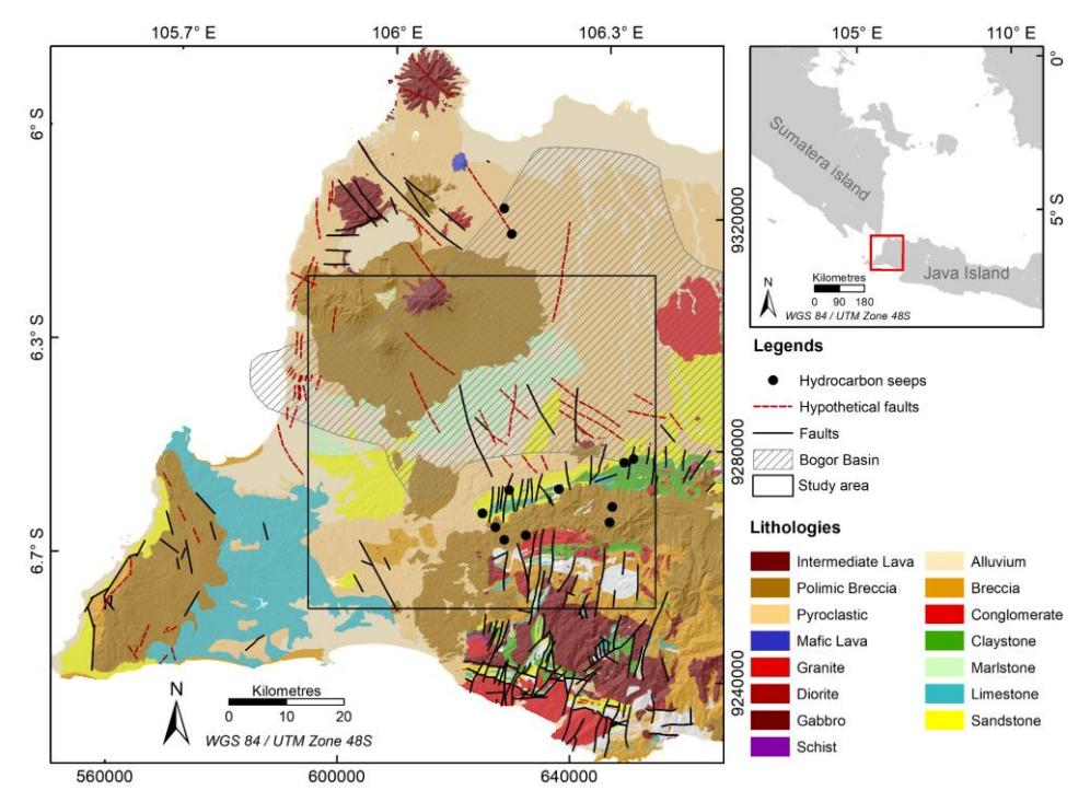
Geological maps in the research area with fault structures and hydrocarbon seeps (modified from Rusmana et al. (1991), Santosa (1991), Sudana & Santosa (1992), as well as Sujatmiko & Santosa (1992)). The Black box in the map is the area of interest for subsurface 3D modelling that includes most of the Bogor Basin zone.
Data and Methods
Gravity Data
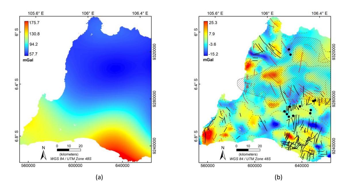
The Earth's gravitational field is an accumulation of various masses contained within the Earth and the structures formed therein. Lithologies and geological structures can be studied based on the density variations of subsurface masses, which are related to the gravity anomaly data measured, as explained by Reynolds (2011) and Telford et al. (1991). The gravity data used in this study were digitized from the Bouguer anomaly maps of Java Island, published by the Geological Survey of Indonesia. The original data have station intervals from 2 to 5 km, as measured by field surveys using a gravimeter. The raw data underwent a standard gravity data processing workflow. The observed gravity data (g_obs) were obtained by applying tidal and drift corrections to the raw data extracted from the instrument. Theoretical gravity values were calculated from normal gravity using the 1967 International Gravity Formula with an ellipsoid reference. Then, free-air (FAC=0.3086h), Bouguer (BC=0.04192ρh), and terrain corrections were applied to produce a complete Bouguer anomaly (Arisbaya et al., 2023; Untung & Sato, 1978). The average rock density of 2.67 g/cm3 was used for Bouguer and terrain correction in the process. The Bouguer anomaly map covering the study area and its surroundings is shown in Figure 2. The Bouguer anomaly ranges from 52.4 to 178.5 mGal, with high values concentrated in the southern part of the study area, particularly in mountainous areas with complex geology, as shown in Figure 1. The northern part is dominated by relatively low uniform values compared to the contrasting anomalies in the south. Qualitative and semi-quantitative analyses were performed over the entire area, as shown in Figures 1 and 2. However, the 3D gravity modelling was focused on the black box area within the coordinate interval from 105.86o to 106.40o in longitude and 6.78o to 6.24o in latitude, covering an area of approximately 60 km by 60 km for time efficiency in the inversion process, as shown in Figure 1.
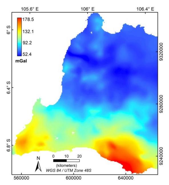
Bouguer anomaly map in the research area from Untung & Sato (1978).
Anomaly Derivatives
In this study, the derivative maps used to delineate the anomaly boundaries and geological structures were HGM, TAHG, and FSED. HGM represents the magnitude of the first-order derivatives of the Bouguer anomaly concerning x and y directions, expressed in Eq. (1) (Cordell, 1979; Ghosh, 2019),
\[HGM = \sqrt{\left(\frac{\partial \Delta g_B}{\partial x}\right)^2 + \left(\frac{\partial \Delta g_B}{\partial y}\right)^2} \tag{1}\]
In the equation, ∆ refers to the Bouguer anomaly. To refine the anomaly boundaries and geological structures that may be subdued due to depth influence, the TAHG technique was employed to facilitate interpretation. The structures can be identified based on the maximum magnitude of the TAHG in the form of radian values ranging from -1.57 to 1.57. TAHG calculation was computed through Eq. (2) (Ferreira et al., 2013),
\[TAHG = \arctan\left(\frac{HGM_Z}{\sqrt{HGM_X^2 + HGM_y^2}}\right)\] (2)
, , and represent the derivatives of HGM in the x, y, and z directions, respectively.
FSED is a more recent edge detection technique than TAHG, utilizing the sigmoid function of the HGM derivatives in the x, y, and z directions. The derivative map produced by this technique can enhance anomaly boundaries and geological structures more effectively, based on their maximum values. The FSED calculation was performed using Eqs. (3) and (4),
\[FSED = \frac{R-1}{1+|R|} \tag{3}\] where,
\[R = \frac{HGM_z}{\sqrt{HGM_x^2 + HGM_y^2}} \tag{4}\]
The ratio between the vertical and horizontal gradients of HGM in the TAHG and FSED mitigates the impact of depth constraint, as the magnitude of deep anomaly boundaries in both the vertical and horizontal gradient will similarly exhibit low values, thereby balancing the magnitudes of both shallow and deep anomalies (Oksum et al., 2021).
Euler Deconvolution
Euler Deconvolution is a mathematical calculation that uses the Euler equation approach to estimate the depth of anomaly sources from potential field data. This technique was first applied to 2D magnetic anomaly sources by
Thompson (1982) and was later developed by Reid et al. (1990) for magnetic sources in a 3D domain. Euler Deconvolution was then more widely utilized for gravity data cases (Marson & Klingele, 1993). Euler deconvolution calculates the relationship between the potential field and its directional derivatives at measurement points (, , dan ) and at the anomaly source locations (0 , 0 , and 0 ) through the 3D form of Euler's equation (Eq. 5),
\[(x - x_0)\frac{\partial \Delta g_B}{\partial x} + (y - y_0)\frac{\partial \Delta g_B}{\partial y} + (z - z_0)\frac{\partial \Delta g_B}{\partial z} = N(B - \Delta g_B)\] (5)
In the equation, N represents the structural index (SI) selected based on the geometry of specific anomalies as described by Reid & Thurston (2014). B is defined as the unknown regional field or a constant background value of the potential field, which can be calculated using the Taylor series approach (Dewangan et al., 2007). The solutions 0 , 0 , dan 0 can be solved by least-square inversion, with the anomaly source locations as the model parameters, as described by Daniel & Kingsley (2020). Reid et al. (2014) stated that the determination of window size and SI greatly influences the results of depth estimation. In this study, the SI used was 0, which represents a simplified geometric approach of thin sheet edges, thin sills, and thin dykes, consistent with the possible geometries formed in the basement due to tectonic and magmatic activities. The appropriate determination of window size must consider several conditions, including being greater than twice the interval between measurement data and greater than half the desired target depth, while being as small as possible. Considering the data intervals range from 2 to 5 km and the target anomaly depth was approximately 9 km (Figure 5), two window sizes were selected for comparison: 7 km x 7 km and 10 km x 10 km. The input data used in this study were residual anomalies, which are considered to no longer contain the regional component of the Bouguer anomaly. Consequently, the depth estimates for the anomalies are expected to be accurately obtained at the boundaries of shallow anomalies.
Gravity Inversion
In this study, we performed the 3D gravity modelling by using Grablox software (Pirttijarvi, 2008). It is a non-linear inversion method for obtaining a subsurface 3D density distribution model from gravity data. The inversion process begins with the discretization of the model area in three directions into blocks with specified dimensions. In addition, density ranges were applied as geological constraints based on the characteristics of the study area. An initial model is then computed by assigning background density values according to the number of defined layers. The optimization of block densities is performed by iteratively applying Singular Value Decomposition (SVD) for matrix inversion. This technique decomposes and attenuates all possible singular values of the inverted matrix, ensuring that the matrix does not reach a singular value (Ren & Kalscheuer, 2020). SVD is highly effective in avoiding ill-conditioned matrix operations, where the matrix tends to have singular values approaching zero, making it impossible for the optimization process to continue (Hansen, 1990).
In addition, the inversion method implements Occam's principle to find the simplest model that fits the data within an acceptable level, usually according to the noise level of the data. In this case, the term "simple" model is associated with a smooth spatial density variation, a smooth interface depth between the upper and lower layers, or both. Therefore, in addition to misfit minimization, the model roughness defined by the spatial difference in the model parameters is also minimized. The iterative process for finding the best model is stabilized by a regularization factor comprising typical depth weighting to avoid near-surface concentration of the anomaly masses (Grandis & Dahrin, 2014; Li & Oldenburg, 1998). The SVD and Occam's inversion processes were repeatedly applied to optimize the vertical extent of the block model. This approach results in a smoother 3D model that is not constrained by the rigid block boundaries. It should be emphasized that inversion modelling, whether using this algorithm or other techniques, is an approach to subsurface modelling. Therefore, it is still possible to apply different techniques and algorithms in the same case study.
Results
Gravity Gradients
The HGM, TAHG, and FSED derived from the Bouguer anomaly are shown in Figure 3, overlaid by the fault structures from the geological map in Figure 1. The maximum magnitudes of the HGM indicate lineaments, suggesting shallow geological structures or anomaly boundaries. Based on the HGM map presented in Figure 3a, the maximum HGM values dominate the southern part of the study area, indicating the presence of anomalies, possibly basement rocks at shallow depths, or geological structures associated with these anomaly boundaries. Most lineaments from HGM do not exhibit maximum values but rather a range between low and high gradient values. Semi-quantitatively, it can be interpreted that the anomaly boundaries or geological structures in the study area are dominated by anomalies at greater depths.
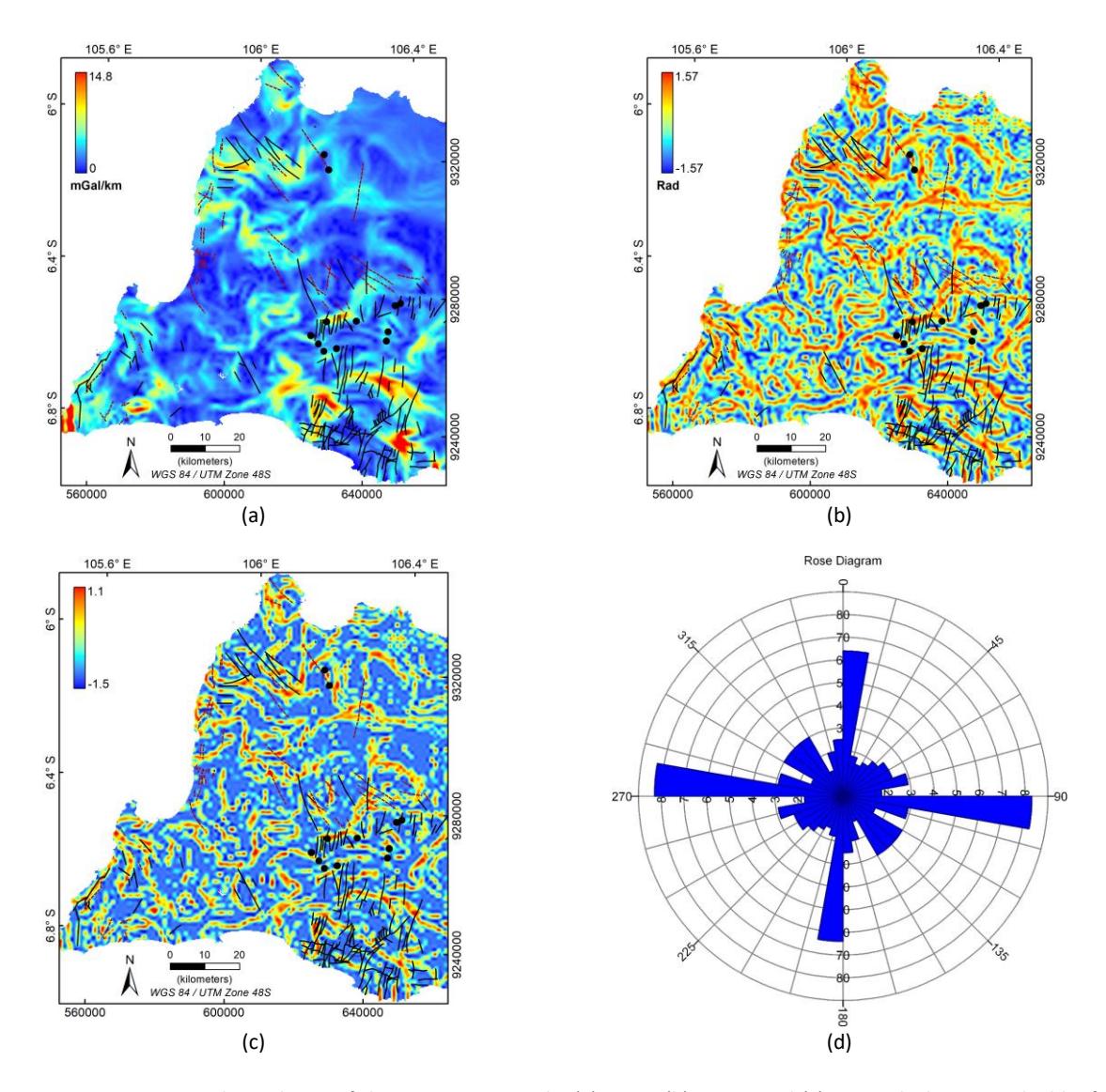
Anomaly gradients of the Bouguer anomaly; (a) HGM, (b) TAHG, and (c) FSED which are overlaid by fault structures from the geological map in Figure 1, as well as (d) the rose diagram of FSED.
The attenuated lineament in the HGM results was enhanced by the TAHG, as shown in Figure 3b. TAHG clarifies lineaments by maximizing all possible geological anomalies and structural boundaries without being influenced by differences in anomaly depths. Based on the analysis results, the TAHG also strengthens the signal from noise, as indicated by the maximum values that do not form lineaments, potentially interfering with the interpretation process. The analysis results demonstrate a better association of fault structures with the maximum values of TAHG than with HGM. The FSED (Figure 3c) produces a sharper gradient contrast at the anomaly boundaries compared to the TAHG, making interpretation easier as the influence of noise is less significant. Based on the comparison with HGM and TAHG, FSED was more effective in mapping anomaly boundaries and geological structures in the study area. Additionally, the correlation of lineaments derived from this gradient is also easier, although generally, FSED still shows gradient patterns similar to those of TAHG.
Some fault structures in the study area were not correlated with the maximum gradients of FSED, except for a few structures, as shown in the figure. This may be because the fault structures in the study area are local, while the gravity data are on a regional and sub-regional scale; thus, the gravity signal does not contain this information in detail. In addition, lineaments do not always indicate the location of fault structures but can also be geological boundaries. However, the lineament trends of the FSED generally illustrate the relationship with the orientation of geological structures in the study area. The results of the lineament trend analysis of the FSED are presented in the rose diagram in Figure 3d. The lineaments of the FSED show north-south and east-west trends that are relevant to the orientation of geological structures in the study area. Furthermore, the location of hydrocarbon seeps correlates with the lineaments from the derivative maps, indicating the presence of fractures as migration pathways for hydrocarbon. The lineaments from the derivative map analysis were then extracted and overlaid onto the residual anomaly to observe the correlation between local anomalies and lineaments.
Depth Estimation of Euler Deconvolution
The results of the Euler deconvolution analysis are visualized on a 2D gridded map, together with the location of the estimated points (Figure 4). The calculation result using a window size of 7 km x 7 km and SI = 0 is shown in Figure 4a. Using these parameters, Euler deconvolution produced depth estimate locations for 3,105 points, which were evenly distributed over the study area and tended to form closed patterns. The calculation results indicated that the anomaly depths varied from 0.7 to 7.3 km. Figure 4b shows the depth estimation map from the calculation using a 10 km x 10 km window size and SI = 0, which produced 2,470 source locations. The distribution of anomaly depth locations using these parameters is relatively relevant to the result of the calculation using a 7 km x 7 km window size. The estimated anomaly depths in this figure range from 0.7 to 5.1 km.
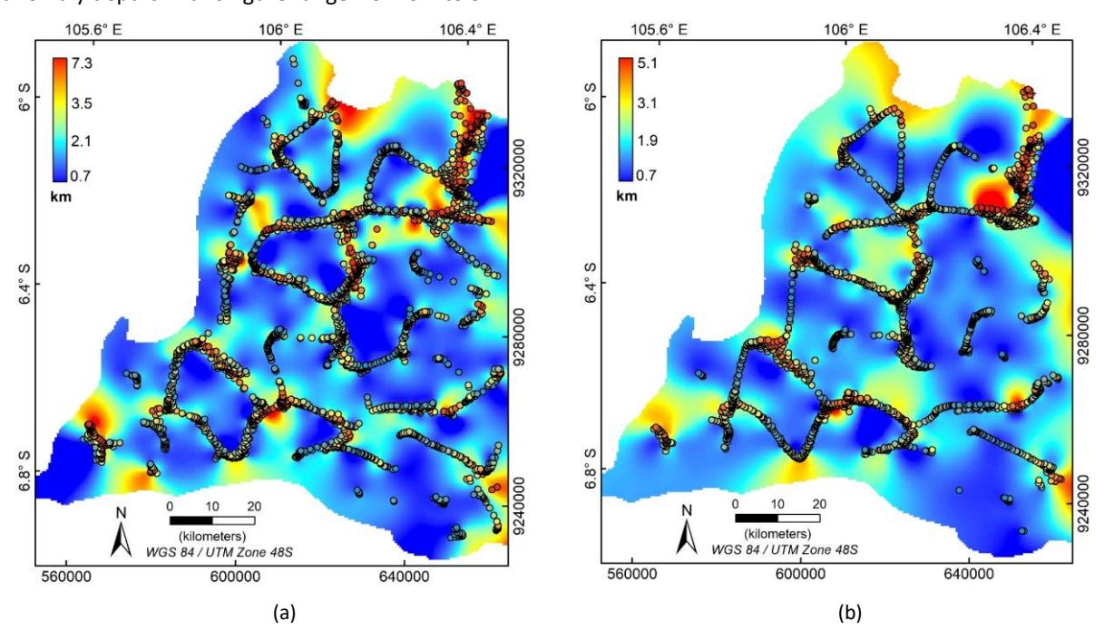
Basement depth estimation of the Euler deconvolution using SI = 0 with (a) window size 7 km x 7 km and (b) window size 10 km x 10 km.
The Euler deconvolution calculations using different window sizes do not show significant differences in the estimated source locations. However, the range of depth estimates obtained showed differences, with larger window sizes estimating shallower anomaly depths. The location of the anomaly sources from these calculations is situated at the boundaries of high and low anomalies of the residual anomaly (Figure 6b), which is also relevant to the anomaly boundaries identified in the gradient analysis (Figure 3). Therefore, it can be concluded that the Euler deconvolution calculations using residual anomaly data are fairly representative for estimating depths at the anomaly boundaries. Further discussion related to the interpretation of the anomaly depths is provided in the Discussion subsection.
Regional and Residual Anomaly
The regional and residual anomalies were separated from the Bouguer anomaly by applying a Butterworth filter (Jensen, 2022; Nafian et al., 2021) with a 50 km wavelength as the anomaly cut-off. This filter can avoid the appearance of Gibb oscillations at discontinuities of separated frequencies, as may appear in lowpass or highpass filters (Saini et al., 2022). Additionally, the estimation of the maximum residual anomaly depth was analyzed based on the results of the Fast Fourier Transform (FFT), followed by the Radially Average Power Spectrum (RAPS) of the Bouguer anomaly, as shown in Figure 5. The results indicate that the maximum depth of the residual anomaly is approximately 9 km.
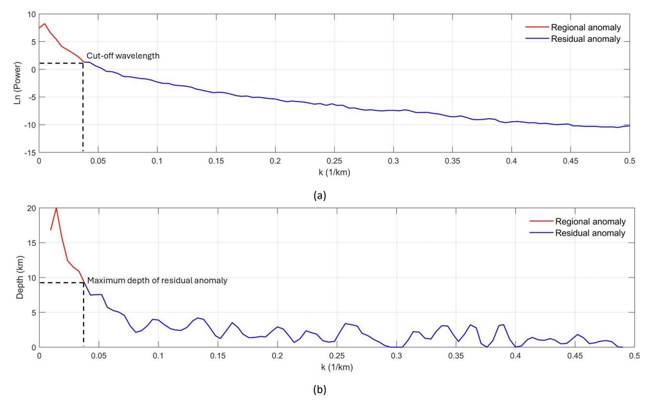
RAPS and depth estimation of the Bouguer anomaly from the result of 2D FFT.
The separated regional and residual anomalies are shown in Figure 6. The regional anomaly in the study area was divided into two regions: a high anomaly in the southern part and a low anomaly in the northern part. The residual anomaly is shown in Figure 6(b), which is overlaid by the lineaments extracted from the analysis of the anomaly gradients and geological information in Figure 1. The distribution of residual anomalies consists of negative anomalies with values ranging from -15.2 to 0 mGal and positive anomalies with a maximum value of 25.3 mGal. The residual anomaly in the Bogor Basin area is predominantly low, which may be associated with the structures that form the basin at greater depths. This is based on the relationship between the gravitational field and the distance from anomalies. In addition, the contrast boundaries between the high and low anomalies largely correlate with the lineaments of the anomaly gradients, as indicated by the brown dashed lines. This suggests that anomaly gradient analysis is highly effective for delineating horizontal lithological boundaries of subsurface anomalies and indicates that the residual anomaly produced at a 50 km wavelength cut-off is appropriate in this case study. The residual anomaly map also shows that several fault structures are associated with the boundaries between positive and negative anomalies, as indicated in the northern and southeastern regions of the study area.
(a) Regional anomaly and (b) residual anomaly overlaid by lineaments from anomaly gradients (dashed brown lines) and the geological information of Figure 1.
3D Inverse Model
Initial Model and 3D Density Model
The initial model was constructed over the study area, measuring 60 km × 60 km with a maximum depth of 10 km, based on the spectrum analysis of the Bouguer anomaly and semi-quantitative interpretation from Euler deconvolution. The inversion block geometry was set at 30 × 30 × 10 blocks, resulting in 18,000 model parameters for the density and height blocks. Each block had dimensions of 2 km × 2 km, with block heights increasing with depth to account for the nearsurface anomaly sensitivity. The sediment density values used represent the average of the geological formations in the study area, which are predominantly composed of limestone (2.55 g/cm³), alluvium (2.0 g/cm³), sandstone (2.35 g/cm³), gabbro (2.7 g/cm³), and granite (2.64 g/cm³), based on the literature by Telford et al. (1991), as well as breccia (2.52 g/cm³) and tuff (2.35 g/cm³), as reported in Legowo et al. (2022) . The density values in the research area ranged from 2.0 to 3.0 g/cm³, based on the estimated lithological variations in the area, as shown in Figure 1. An illustration of the constructed initial model is presented in Figure 7. The data used in the modelling process (observed data) were the residual anomalies in the study area.
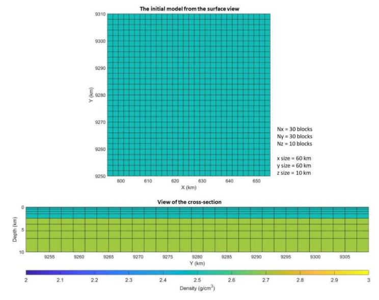
The initial model for the inversion process had two density layers.
The result of 3D modelling is shown in Figure 8a as a 3D density model. The final Root Mean Square (RMS) error of the modelling processes is 0.028 mGal based on the misfit of the calculated (Figure 8(c)) and observed data (Figure 8(b)) as input, while the model RMS for Occam to SVD is 0.0037 g/cm3after three iterations. Based on the obtained 3D model, 2D cross-sectional models are also presented along profiles A and B with the responses of the calculated and observed data (Figures 9(a) and 10(a)). The 2D cross-section along profile A shows a reasonably good relationship between the observed and calculated data with an RMS error of 1.05 mGal, and the cross-section along profile B has an RMS error of 0.71 mGal. The 2D cross-sections yielded smooth density models (Figures 9(b) and 10(b)), as expected from the Occam inversion results. Further analysis and interpretation are discussed in their respective subsections.
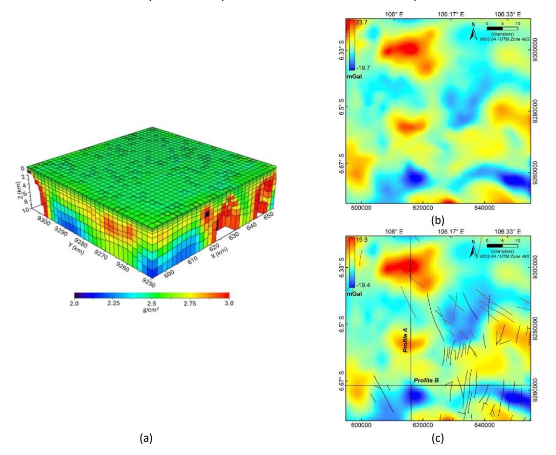
(a) The result of the 3D density model based on the SVD and Occam inversion, (b) the observed data in the study area of modelling, and (c) the calculated data of the model.
Discussion
Subsurface Cross-sections
The 2D cross-section of profile A is depicted in Figure 9b, which illustrates three high-density anomalies as the basement layers, i.e., HD-1, HD-2, and HD-3. Low densities, ranging from 2.05 g/cm3 to 2.7 g/cm3 , are interpreted as the accumulation of sedimentary layers above the basement rock. The section is also overlaid by the estimated basement depth curve from Euler deconvolution calculations and fault structures interpretation based on geological information. Figure 8c indicates that the 2D cross-section of profile A intersects two structures identified as lineaments based on aerial imagery from the Geological Map of Serang by Rusmana et al. (1991). The lineaments are depicted as black lines on the model, with dashed extensions to account for the depth ambiguity of the structures.
Based on the 2D cross-section, the lineaments can be identified as fault structures due to their location in the discontinuity between two basement rock layers (HD-2 and HD-3). This area also lies within a low-density zone with a relatively lower density than its surroundings. The zone can be identified as a sedimentary basin along a distance of 9277-9300 km. The sedimentary basin area interpreted from the model is part of the Bogor Basin, which extends along a distance of 9272-9308 km. The model indicated that the maximum depth of the basin reached 5 km, with the potential for greater depths of up to 10 km. This result demonstrates that the Bogor Basin can be effectively identified in the gravity modelling results.
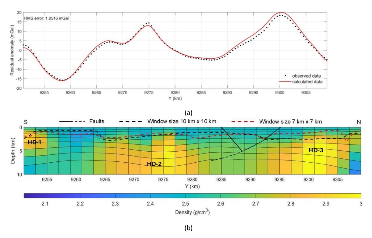
(a) Comparison of observed-calculated data and (b) interpretation of the cross-section on profile A; dashed lines are the depth estimation of the Euler deconvolution.
The depth estimations derived from the Euler deconvolution results did not show significant differences. Both indicated depth variations ranging from 1 to 3 km, with comparable depth trends. Nevertheless, a discrepancy is evident between the two results at the sediment-basement interface of HD-3. The Euler calculation with a window size of 10 km x 10 km (black dashed line) is more representative of this interface than the 7 km x 7 km window size (red dashed line). However, the Euler depth estimations did not indicate any discontinuities between the HD-1 and HD-2 anomalies or within the basin between HD-2 and HD-3, as illustrated by the resulting density model.
The geological map of Serang demonstrates that the pyroxene andesite-basalt rock formation in the Karang Mountain area is associated with the HD-3 high-density anomaly. Subsequently, sediments from the Karang volcanic product and the Bojong Formation, composed of sandy marl, sandy clay, and tuffaceous sandstone, accumulated on top of bedrock in the zone. The southern area of the cross-section contains sediment accumulation consisting of the Bojongmanik and Cipacar Formation, as indicated on the geological map of the Leuwidamar by Sujatmiko & Santosa (1992).
Profile B traverses numerous north-south oriented fault structures, as shown in Figure 8(c). The faults intersected by this section include both strike-slip and normal/reverse faults, based on information from the Leuwidamar Geological Map by Sujatmiko & Santosa (1992). The dip direction of the faults was adjusted to match the dip of the basement model in a 2D cross-section, with the surface fault coordinates aligned with geological information. Three high-density anomalies, HD-1, HD-2, and HD-3, observed in the 2D cross-section of profile B (Figure 10(b)), are interpreted as a single unit of basement rock experiencing discontinuities. These discontinuities form a basin between the high anomalies HD-2 and HD-3 with the existence of six fault structures, which may extend to a depth of 10 km. The dashed black lines on these fault structures indicate uncertain depths due to the continuity to greater depths. The presence of complex fault structures in this basin can indicate potential hydrocarbon accumulations, as evidenced by hydrocarbon seep manifestations near profile B. Additionally, the HD-1 anomaly forms a basin down to a depth of approximately 4 km, containing two fault structures in that zone.
The estimated basement depths from Euler deconvolution with varying window sizes exhibit a comparatively consistent depth curve pattern along profile B (Figure 10(b)). The depth estimations demonstrated a relatively good correlation with the sediment-basement boundary in the 2D cross-section of the profile. In the shallow basin identified at HD-1, the depth estimation using the 10 km x 10 km window size (black dashed line) correlates more closely with the sedimentbasement interface of the density model than the 7 km x 7 km window size (red dashed line). However, the Euler depth
estimations did not indicate any discontinuities between the high anomalies, either between HD-1 and HD-2 or between HD-2 and HD-3. This condition may occur because the depth estimation approach using Euler deconvolution only approximates the source depths at the anomaly boundaries, not the entire interface of the sedimentary layer and basement, as shown in Figure 4. However, it is still possible to use semi-quantitative Euler calculations for depth estimation in this case study, although the approach is relatively coarse and less accurate.
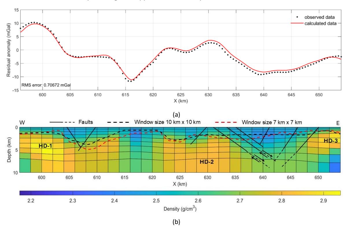
(a) Comparison of observed-calculated data and (b) interpretation of the cross-section on profile B, dashed lines are the depth estimation of the Euler deconvolution.
Based on the Geological Map of Leuwidamar, the sedimentary deposits that overlay the bedrock in profile B exhibit remarkably intricate variation, particularly in the eastern section. The area is composed of various sediments, including citorex tuff, which is characterized by a rock composition of breccia, mudstone, lava, sandstone, and claystone. Additionally, the Badui Formation and the Cimapag Formation are present, which are comprised of rock types such as conglomerate, breccia, tuff, and sandstone. In the western part above the HD-1 anomaly, various sediments accumulated from the Endut Volcano Formation, consisting of volcanic breccia, lava, and tuff, as well as the Malingping Tuff Formation with rock types of breccia, pumice, lava, sandstone, and claystone.
Basement Depth Map
In addition to the depth interpretation of the basement rock from the 2D cross-sections along profiles A and B, the basement depth was also visualized in the form of a map derived from the 3D density model. The basement was interpreted at a density of 2.8 g/cm³, marking the boundary with the overlying sedimentary layers. The depth of the basement at this density boundary is shown in Figure 11. The basement depth based on the 3D density model in the study area varied from 0.2 km to 7.8 km. However, the maximum depth could exceed 10 km, as 2D cross-sections indicate basins extending beyond this depth. The maximum depth boundary shown in Figure 11 is an interpolation of the basement depth that can be identified at this density cut-off.
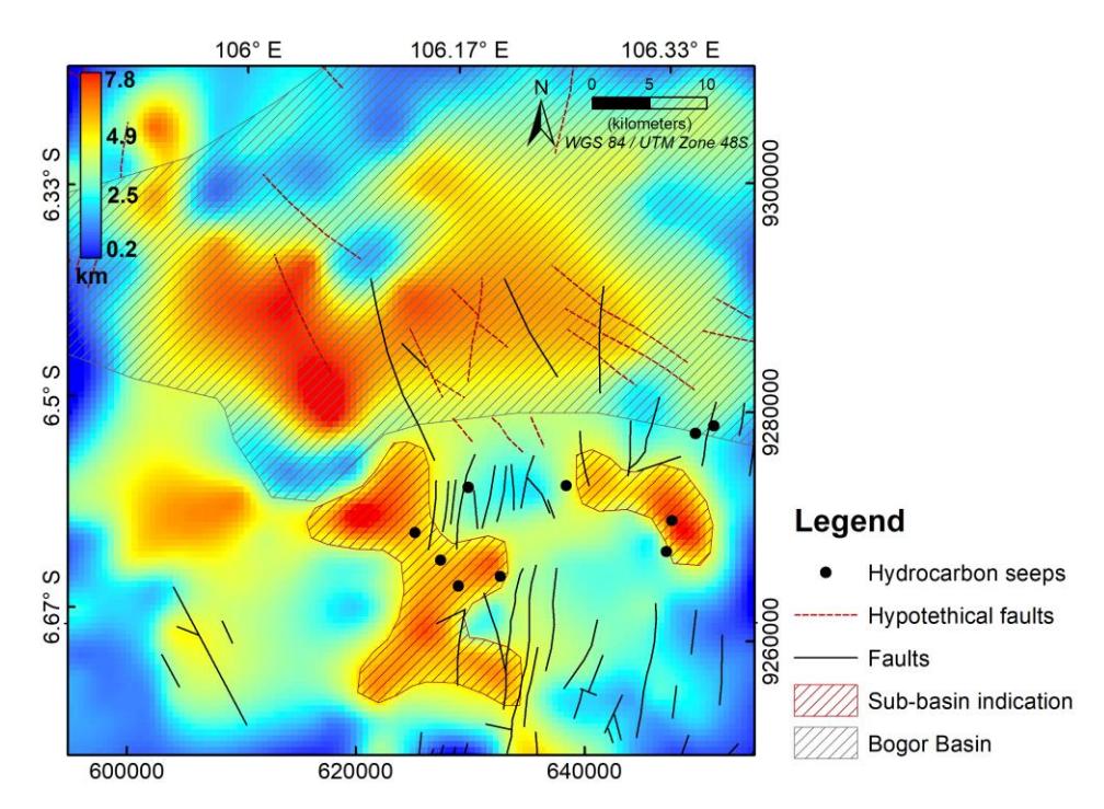
Depth to basement map extracted from 3D density model at a 2.8 g/cm3 density cut-off.
The basement depth map (Figure 11) in the study area reveals regions of significant depth that correlate with the Bogor Basin area. The deep basement in this region can be interpreted as the Bogor Basin, which is also associated with fault structures, although some parts of the basin have relatively shallower depths. The indication of the Bogor Basin from the basement depth map is consistent with the distribution of low residual anomaly (Figure 6b) in the same area, as a consequence of the basement anomalies at greater depths. This correlation suggests that the basin geometry can be semi-quantitatively estimated from the distribution of residual anomalies, particularly at its lateral boundaries. In the southern part of the Bogor Basin, as shown in Figure 11, there are indications of sub-basins associated with complex fault structures and hydrocarbon manifestation points. Hydrocarbon manifestations at the surface tend to occur outside the Bogor Basin, which is reasonable because of the complex fault structures that serve as migration pathways for hydrocarbons formed in the basin.
Conclusion
Based on the comparison of several derivative maps, we conclude that FSED is the most effective tool for detecting anomaly boundaries and geological structures from gravity data. It enhances the boundaries of anomalies that are damped due to the depth effect of HGM results and provides sharper anomaly boundaries than the results from TAHG. The mapped anomaly boundaries from FSED also correlated well with the high and low anomaly boundaries from the residual anomaly. In addition, some fault structures and hydrocarbon seep locations are also correlated to the lineaments of the anomaly gradients, but most of the localized structures cannot be identified, which may be due to the influence of measurement spacing that is unable to record the gravity signal in detail.
Depth estimation of anomalies based on Euler deconvolution calculations using different window sizes does not show significant differences in the estimated location of anomaly boundaries and depth curves on profiles A and B. Based on the comparison to 2D density models of profiles A and B, the depth estimation results show a good correlation with the interface of the sediment and basement layer. In some areas, the depth estimation using a 10 km x 10 km window size correlates more closely with the models than the 7 km x 7 km window size. The basement depth map from the 3D density model indicates the presence of a basin within the Bogor Basin area, as well as sub-basins in the southern part, which are associated with complex fault structures that could potentially serve as hydrocarbon migration pathways. These basin structures are also evident in the 2D cross-sections of profiles A and B. The lateral boundaries of these basin structures correlate with low residual anomalies, suggesting that the lateral boundaries of the basins can be roughly estimated semi-quantitatively.
Acknowledgment
The Educational Fund Management Institution or LPDP, Ministry of Finance Indonesia, provided scholarships to Riski Ananda and Tony Rahadinata for their study in the master's program at Institut Teknologi Bandung. Continuous support from the Institute for Research and Community Services (now Directorate of Research and Innovation) ITB through various research grants is highly appreciated.
Compliance with ethics guidelines
The authors declare they have no conflict of interest or financial conflicts to disclose.
This article contains no studies with human or animal subjects performed by the authors.