1 Introduction

Quantisation is the process of approximating the continuous range of signal value by relatively small of integer values. The input of the quantiser is the original data and the output is within a finite number of levels. Good quantiser is one which represents the original signal with minimum loss or distortion.

The quantiser output may be encoded using variable-length or fixed-length code words due to the fact that when we code a word, we do not have to have equal number of bits. Similarly, when we quantise a signal, we do not have to have equal length of quantise.

In general, there are two types of quantisation, i.e., scalar and vector quantisations. In scalar quantisation, each input symbol is treated separately in relation to its output, whereas in vector quantisation the input symbols are grouped together in vectors, and processed to give the output. The upside part of this data grouping scheme is due to the optimality increases of the vector quantiser, but at the cost of increased computational complexity.

A quantiser also can be specified by its reproduction points. If the input range is divided into levels of equal spacing, then the quantiser is termed as a uniform quantiser, and if not, it is termed as a non-uniform counterpart. A non uniform one has smaller quantisation step for small input and vice versa.

A uniform quantiser can be easily specified by its lower bound and the step size. Also, implementing a uniform quantiser is easier than a non-uniform quantiser. Interested readers may refer to [1-4].

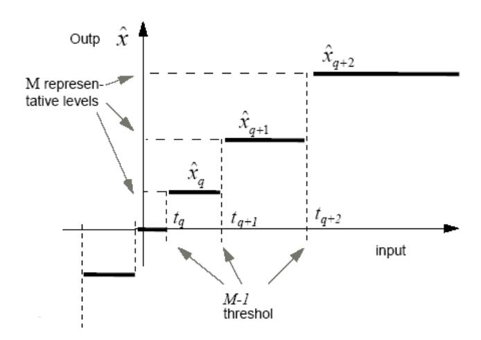
Figure 1 Typical Input Output Characteristic of a Scalar Quantiser.

Scalar quantisation is the process of mapping an input value, x, into a finite number of output value y, given by Q : x → y ; see Figure 1 for its input-output characteristics. The difference between the actual analog value and digitally quantised value is called quantisation error. This is due to rounding or truncation. In this paper, we shall investigate two practical scalar quantisers (Lloyd-Max and the uniformly defined one) and compare their performances against Shannon's limit R. The unit for R is bits/sample.

The organisation of this paper is as follows. Firstly, several backgrounds related to information theory and the organisations of this paper are introduced in Section I. In Section II, the performances of Lloyd-Max scalar quantisers against its Shannon limit are depicted. Entropy coded of a uniform quantiser is given in Section III. In order to investigate how close we can get to the entropy H using Huffman coding scheme, its performances are also depicted in Section IV. Discussion and conclusions are accordingly drawn in last section.

2 Source Coding Theorem

Source Coding Theorem, known as noiseless coding theorem, establishes the limits to possible data compression. The theorem itself, proved by Shannon's in 1948, only gave necessary and sufficient conditions for the existence of the source code. It does not provide any algorithm for the design of codes that achieve the performance predicted by this theorem.

In the case of a continuous source, the question is how we represent it with finite R bits/symbol. In theory, it has infinite precision which implies infinite entropy. In representing the source output in finite discrete form, we tacitly accept a certain amount of distortion (or quantisation error). The question then is if we represent the source output by finite R bits/symbol, how close can the compressed version and the original version be? Again, it was Shannon who did the momentous work shown below. Let X be the source output, and Xˆ its reproduction. In the continuous case, we often measure the distortion by the square-error distortion defined by:

\[d(X,\hat{X}) = (X - \hat{X})^{2}.\] (1)

(Not always, Hamming distortion is equally popular in communication theory). Regarding (1), since the source output is a random variable, d(X,Xˆ) is also a random variable, we therefore define the average distortion as the expected value:

\[D = E[d(X, \hat{X})].\]

Shannon's Rate-Distortion Theorem states as follows: the minimum number of bit/source output required to reproduce a memory-less source with distortion less than or equal to D is called rate-distortion function, denoted by R(D) and given by:

\[R(D) = \min_{p(\hat{x} \mid x) : Ed(X, \hat{X}) \le D} I(X; \hat{X}),\] where \(I(X; \hat{X})\) denotes the mutual information between X and \(\hat{X}\). \(p(\hat{x} \mid x)\) is the conditional probability function which the code designer must find in order to achieve the optimum result.

The proof for the general theorem is too involved to be shown here. Shannon in the same paper derived the rate-distortion function for Gaussian source with variance \(\sigma^2\) as an example:

\[R(D) = \begin{cases} \frac{1}{2} \log \frac{\sigma^2}{D} & 0 \le D \le \sigma^2, \\ 0 & otherwise. \end{cases}\]

The distortion measure is square-error as defined above. Interested readers are suggested to referred to [1-2] and [4-7] for details.

The main objective, in this context, is to design the optimum code. The full understanding of the theorem also helps in setting the direction to achieve such an optimum result. Interested readers may refer to [8-16] for a more comprehensive explanation.

2.1 Optimum Scalar Quantisation – Lloyd-Max Quantiser

Given a positive definite Gaussian function as follows (see Figure 2):

\[p_x(x) = \frac{1}{\sqrt{2\pi\sigma}} \exp(-x^2/2\sigma^2).\]

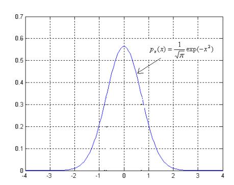
Figure 2 Sample of Gaussian Pulse with \(\sigma = 1/\sqrt{2}\).

Accordingly, the decision levels \(x_k\) and the reconstruction values \(y_k\) for the Lloyd Max quantiser for L=2, 4, 8, 16, 32 and also 64 levels can be calculated using the equations (2) and (3).

As a result, the reconstruction value can be calculated by equation (2).

\[y_{k} = \frac{\int_{x_{k}}^{x_{k+1}} x.p_{x}(x)dx}{\int_{x_{k}}^{x_{k+1}} p_{x}(x)dx}, \text{ k=1, 2... L}\] (2)

The decision threshold is exactly halfway between its representative levels:

\[x_k = \frac{1}{2}(y_k + y_{k-1}) \text{ k=2, 3... L}\] (3)

The positive definite function (pdf) of the weighted quantisation errors for each decision interval \(l_k\) is given by:

\[\sigma_k^2 = \int_{x_k}^{x_{k+1}} (x - y_k)^2 p_x(x) dx.\] (4)

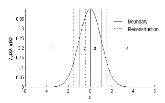
Figure 3 Optimum Quantiser (by Lloyd Algorithm).

The above equations must be solved numerically using iterative algorithm. Firstly, an arbitrary initial sets of \(x_k\) and \(y_k\) were chosen. The optimum

solution must satisfy equation (2). This process was iterated until the difference between two successive approximations is below a threshold value.

The problem of designing a quantiser is to determine the optimum decision \(x_k\) and reconstruction levels \(y_k\) for a given \(p_e(e)\) optimisation criterion given by Figure 3. Thus, the average distortion is \(D = \sigma_q^2\), where:

\[\sigma_q^2 \stackrel{\Delta}{=} \sum_{k=1}^L \int_{x_k}^{x_{k+1}} (x - y_k)^2 p_x(x) dx,\] \[= \varepsilon_*^2 2^{-2R} \sigma_x^2.\] (5)

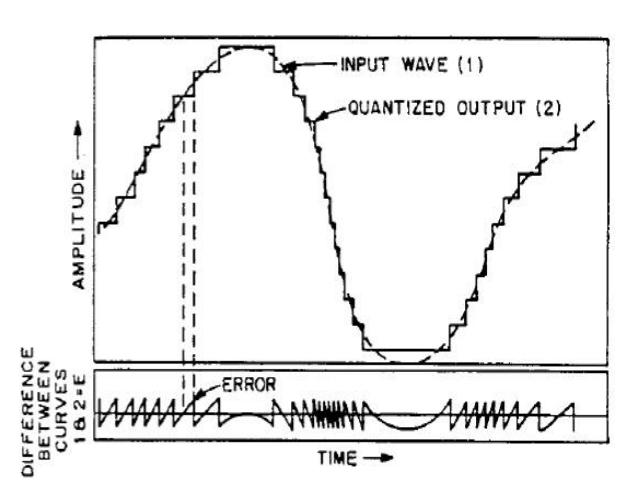
Figure 4 An Example of Quantized Waveform.

As depicted by Figure 4, the quantised output is the replicate of the input wave. However, due to some errors known as quantisation errors, they may not create an exact copy of its input wave.

2.2 Quantiser Performances

The overall calculations were solved by Matlab iteratively. However, some manual calculation will be initially given.

For L=2

In order to simplify the calculation, it is assumed that \(\sigma = 1/\sqrt{2}\). As a result, we end up with the following Gaussian function:

\[p_x(x) = \frac{1}{\sqrt{\pi}} \exp(-x^2).\]

As a result, according to (2) the reconstruction values become:

\[y_{k} = \frac{\int_{0}^{\infty} x \frac{1}{\sqrt{\pi}} \exp(-x^{2}) dx}{\int_{0}^{\infty} \frac{1}{\sqrt{\pi}} \exp(-x^{2}) dx},\] \[= \frac{\left[-\frac{1}{2}e^{-x^{2}}\right]_{0}^{\infty}}{\left[\frac{\sqrt{\pi}}{2} \operatorname{erf}(x)\right]_{0}^{\infty}}.\] (6)

Due to the fact that \(\operatorname{erf}(\infty) = 1\) and \(\operatorname{erf}(0) = 0\), we finally end up with \(y_k = 0.5642\) for L=2. Since we choose to \(\operatorname{employ} \sigma = \sqrt{2}\), we need to renormalise \(y_k\) to \(\sqrt{2}\). Accordingly, the final value of \(y_k\) for L=2 becomes, \(y_k = 0.5642\sqrt{2} = 0.7979\).

The calculation of \(y_k\) for L=4 up to L=32, can be found iteratively using (2) and under the assumption that \(x_{k+1} = 1\), we eventually obtain equation (7).

\[y_{1} = \frac{\left[-e^{-x^{2}}\right]_{0}^{x=x_{1}}}{\sqrt{\pi} \cdot \left[erf(x)\right]_{0}^{x=x_{1}}},\] \[= \frac{(1-e^{-x^{2}})}{\sqrt{\pi} \cdot (1-erf(x_{1}))}.\] (7)

Subsequently,

\[y_2 = \frac{e^{-x_1^2}}{\sqrt{\pi} (1 - erf(x_1))}\]

Thus, the decision levels can be calculated as follows:

\[x_k = \frac{1}{2}(y_k + y_{k-1}),\]

accordingly,

\[x_1 = \frac{1}{2}(y_1 + y_2).\]

The result is iteratively computed using (7).

Probability of Error

To compute the probability of error, we begin with:

\[P_{k} = \int_{x_{k}}^{x_{k+1}} p_{x}(x) dx \tag{8}\]

As a result, \(P_k = \int_{x_0}^{x_{k+1}} \left[ \frac{1}{\sqrt{2\pi}\sigma} \exp(\frac{-x^2}{2\sigma^2}) \right] dx\), due to \(\sigma^2 = 1/\sqrt{2}\), the equation in (8)

finally becomes:

\[P_{k} = \frac{\sqrt{\pi}}{2\sqrt{\pi}} \left[ erf(x) \right]_{x_{k}}^{x_{k+1}},\]

\[P_k = \frac{1}{2} \left[ erf(x) \right]_{x_k}^{x_{k+1}},\]

\[=\frac{1}{2}[erf(x(k+1)-x(k))].\]

In Matlab, the error function erf(x) is given by twice the integral of the Gaussian distribution curve with zero mean and variance of 0.5 as given by:

\[erf(x) = \frac{2}{\sqrt{\pi}} \int_0^x e^{-t^2} dt.\] (9)

Signal Power

If x corresponds to signal on one ohm resistor, then \(x^2\) represent the power of that particular signal. Hence the statistical average of power is given by:

\[\overline{x^2} = \int_{-\infty}^{\infty} x^2 p(x) dx = \sigma^2 = 1.\] (10)

Matlab Simulation

The algorithm applied in Matlab to compute the values of \(x_k\) and \(y_k\) can be depicted as follows. Firstly, the number of decision level, L, and the initial value of \(x_k\) and \(y_k\) are given. Accordingly, the new representative levels and decision threshold are iteratively computed, the computational results are convergent enough until the value of threshold is reached. Otherwise, the iteration has to be stopped. In short, it is given in flowchart in Figure 5.

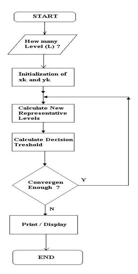
Figure 5 Matlab Iterations to obtain \(x_k\) and \(y_k\).

2.2.1 Computation Results

The Matlab computational results in terms of x(k), y(k) and the probability of error Pe (from L=2 to L=64) are graphical represented in Figures 6-8. As can be seen, the reconstruction values ^k y increase proportionally to the values of k, see Figure 6. Figures 6-10 and Figure 12 are obviously discrete events. The continuous lines on the graphs are only meant to indicate the trend.

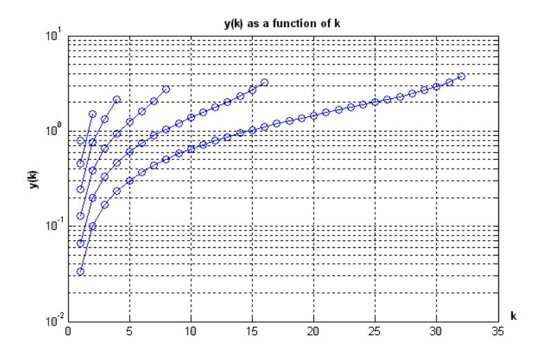
Figure 6 The Reconstruction Values vs. k.

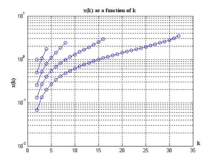
Figure 7 Decision Levels against k.

Correspondingly, the decision levels x(k) obviously follow that pattern and given by Figure 7.

The last decision level x(k) is always located in infinity; therefore, they cannot be shown in Fig 8. Also for L=2, x (1) =0 and x (2) =infinity.

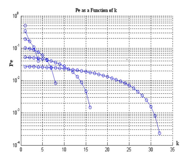
Figure 8 Probabilities against k in Semi-Log Scale .

Figure 8 apparently indicates that P^k associated with interval is not identical. It decreases as the value of k increases. In other words, they are inversely proportional to k.

In addition the pdf weighted quantisation errors are almost identical except for the last interval as given by Figure 9.

Accordingly, the error variance contributions ^{2 σ k} are almost the same for all intervals k=1, 2… L, see [1] for more comprehensive explanations. The last interval is indeed not typical of the systems.

Figure 10 depicts the average distortion as a function of bit rate R. It turns out that the smaller the interval, the less quantisation noise or distortion is going to exist. Distortion decreases by factor 4 (6 dB) every increase of one bit coding.

Click to buy NOW!

^www.docu-track.co^m

^PDF-XCHANG^E

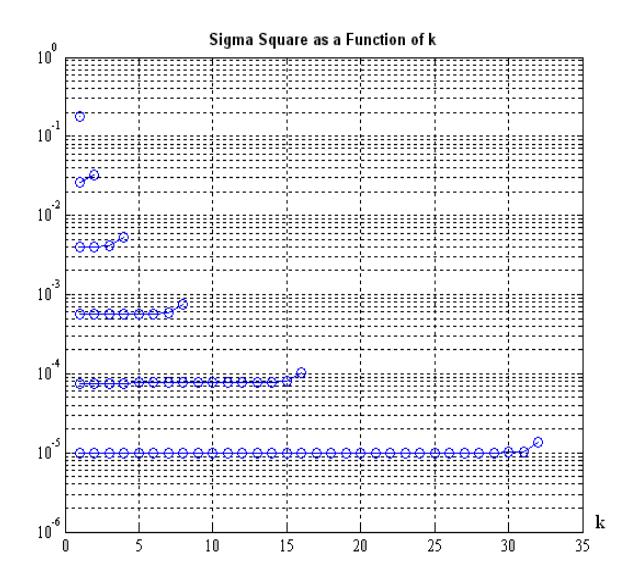
Figure 9 The pdf weighted quantisation Error Against k .

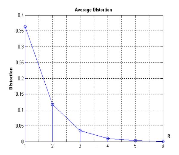
Figure 10 Average Distortion as a Function of R.

In some cases, transmitting at rate close to entropy is not possible. For instance when the entropy of the information is greater than storage capacity, error is indispensable. In this case, some lossy compression technique must be employed and some distortion will be introduced accordingly. It calculates the minimum transmission bit rates R, for a required picture quality.

Figure 11 Image Transmission.

Figure 11 depicts the process of image transmission. A distortion can be defined as a distance between x and its reproduction %, denoted by d(x, %). In the discrete time system Hamming distortion is commonly used. It is depicted as follows:

\[d_H(x,\hat{x}) = \begin{cases} 1, & (x \neq \hat{x}) \\ 0, & otherwise \end{cases}\] (11)

Whereas in the continuous case, the squared distortion is expressed as follows:

\[d(x,\hat{x}) = (x - \hat{x})^2 \tag{12}\]

Also, the average distortion can be defined as the expected value

\[D = E[d(X, \hat{X})] \tag{13}\]

Rate-distortion form is often used to measure the quantiser performance as given by:

\[\sigma_q^2 \stackrel{\sum}{=} \sum_{k=1}^{L} \int_{x_k}^{x_{k+1}} (x - y_k)^2 p_x(x) dx = \varepsilon_*^2 2^{-2R} \sigma_x^2\] (16)

where \(L=2^R\) is the number of levels, \(\sigma_x^2\) corresponds to signal power.

\[\sigma_x^2 = \overline{x^2} = \int_{-\infty}^{\infty} x^2 p(x) dx = \sigma^2 = 1\] (17)

Then the performance factors are given as follows:

• \(\varepsilon_*^2 = 4.5\) for laplacian positive definite function (pdf),
• \(\varepsilon_*^2 = 1.0\) for uniform distributed pdf and
• \(\varepsilon_*^2 = 2.71\) for gaussian pdf.

Shannon derived the rate distortion function for Gaussian source with variance \(\sigma^2\) as:

\[R(D) = \begin{cases} \frac{1}{2} \log \frac{\sigma^2}{D} & 0 \le D \le \sigma^2 \\ 0 & otherwise \end{cases}\] (18)

Moreover,

\[SNR = \frac{\sigma_x^2}{\sigma_\varrho^2} = \frac{\sigma^2}{D}.\] (19)

The inverse relationship for (19) is given by:

\[D = 2^{-2R} \sigma^2\], (20)
\(SNR = 2^{2R} = \sigma^2 / D\).

By taking 10-based-logarithmic to convert (20) into dB, we finally obtain:

\[SNR = 10^{10} \log_2(2^{2R}) ,\] \[= 10^{10} \log_2 \frac{\sigma^2}{D} ,\] \[= 20R \log 2 ,\] \[= 6.03R .\]

Accordingly, Shannon Rate Distortion (in log 10) is given by:

\[R = SNR / 6.03\] (21)

Inverse of the above equation is given by: \(2^{2R} = \sigma^2/D\). However, as already defined \(\sigma^2/D = SNR\), accordingly, Shannon Rate Distortion (in log 2) is given by:

\[R = \frac{1}{2}\log_2(SNR). \tag{22}\]

The average distortion \(D = \sigma_q^2\) is identical to the average quantisation noise.

The quantiser output can be regarded as a discrete-valued memory less source with L-ary alphabet. The entropy \(H_{\mathcal{Q}}\) for different quantisation levels is depicted as follows:

\[H_{Q} = -\sum_{k=1}^{L} P_{k} \log_{2} P_{k}. \tag{23}\] in which \(P_k\) corresponds to the probability within the interval k, and rely on the chosen decision regions. Figure 12 shows that entropy increase linearly proportional to R.

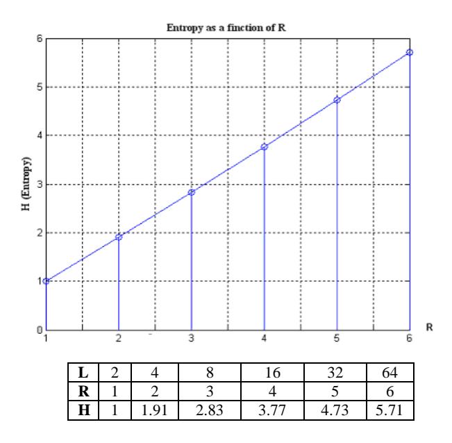
Figure 12 Entropy as a Function of R (in a linear scale).

Graphical representation of entropy-distortion characteristic of the Lloyd-Max quantiser from L=2 to up to 64, with the Gaussian positive definite function is given by Figure 13.

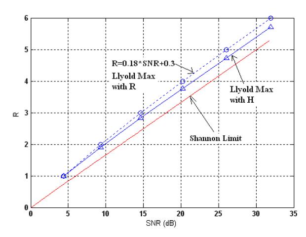
Figure 13 Optimality Comparison of Lloyd Max Quantiser to Shannon Limit

It turns out that at lower R Lloyd's SNR is getting closer and approaching to its Shannon limit. On the other hand, at higher R, its SNR is getting farther below Shannon Limit, say, for instance R=5, the difference is reasonably big, more than 4 dB.

It is now apparent that from the set of numerical data, theoretical Shannon limit only can be closely approached. It cannot be surpassed irrespective of the coding schemes applied.

3 Entropy-Coded Uniform Quantiser

The length of the interval was chosen in such a way that \((L/2)\Delta = 3\sigma\). If \(\sigma = 1\) then \(L = 6/\Delta\). The simulation result from Matlab is given below. \(x_k\) (the decision level) is selected to be uniformly apart and the value of L is arbitrary.

Hence, the average bit rate is given by \(\overline{R} = \sum_{i=1}^{n} P_i b_i \neq \log_2 L\). Then \(y_k\) as the reconstruction value still to be the centroid of quantisation interval, in order to minimise the quantisation noise within the interval. Again, in practice, Figures 14-15 obviously occur in discrete domain. The continuous lines are only meant to point out the trends.

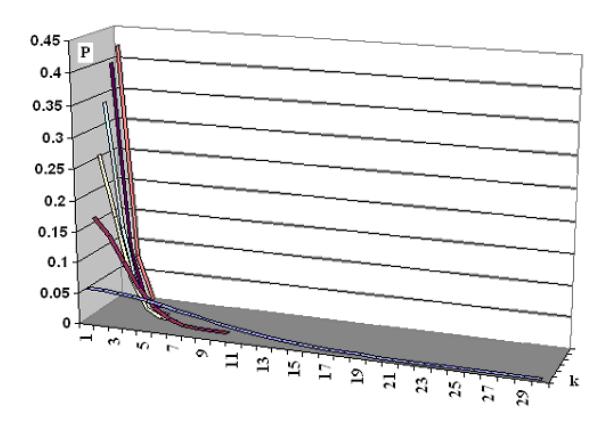
Figure 14 Probability as a Function of k (Linear Scale).

Figure 14 points out that the value of P(k) decrease as the number of k increase, the smaller the value of k the bigger the value of P(k) and vice-versa.

As it has already been depicted in part one the value of y(k) increase sproportionally to the number of k. Nearly, of each interval the position of y(k) is in the halfway between x(k).

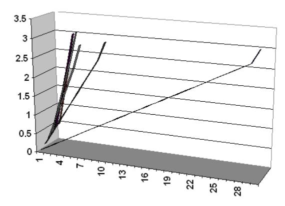
Figure 15 y(k) Against k in Linear Scale.

3.1 Huffman Code

Huffman codes provide a prefix code with minimum average block length. The algorithm is given in the flowchart in Figure 16.

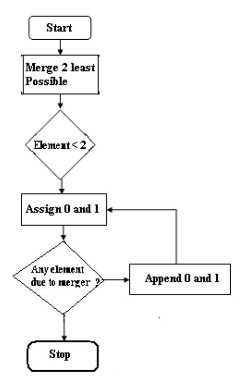
Figure 16 Flowchart of Huffman Coding Algorithm.

Its code tree can be obtained as follows:

• The two symbols with the lowest probability are picked and merge into a new auxiliary symbol.
• The probability of merged symbol is calculated
• If more than 2 symbols remain, then, repeat the first two steps for the new auxiliary alphabet
• The code tree is converted into prefix word.

Matlab Syntax to perform Huffman Coding Automatically:

DICT = HUFFMANDICT(SYM, PROB)

In which, Sym represent symbols that are used, and prob corresponds to probability of them. For instance, when Delta=0.3, L=20 the results (code books) are given as follows

dict =
 [-3.0058] [1x13 double]
 [-2.5311] [1x12 double]
 [-2.2333] [1x10 double]
 [-1.9355] [1x8 double]
 [-1.6377] [1x6 double]
 [-1.3399] [1x5 double]
 [-1.0422] [1x4 double]
 [-0.7444] [1x3 double]
 [-0.4466] [1x3 double]
 [-0.1489] [1x3 double]
 [ 0.1489] [1x3 double]
 [ 0.4466] [1x3 double]
 [ 0.7444] [1x3 double]
 [ 1.0422] [1x4 double]
 [ 1.3399] [1x5 double]
 [ 1.6377] [1x5 double]
 [ 1.9355] [1x7 double]
 [ 2.2333] [1x9 double]
 [ 2.5311] [1x11 double]
 [ 3.0058] [1x13 double]
 -3.0058 <1x13 double>
 -2.5311 <1x12 double>
 -2.2333 [1 1 1 1 0 1 0 1 0 0]
 -1.9355 [1 1 1 1 0 1 0 0]
 -1.6377 [1 1 1 1 0 0]
 -1.3399 [1 1 1 0 1]
 -1.0422 [1 0 0 1]
 -0.7444 [1 1 0]
 -0.44664 [0 1 1]
 -0.14888 [0 0 1]
  0.14888 [0 0 0]
  0.44664 [0 1 0]
  0.7444 [1 0 1]
  1.0422 [1 0 0 0]
  1.3399 [1 1 1 0 0]
  1.6377 [1 1 1 1 1]
  1.9355 [1 1 1 1 0 1 1]
  2.2333 [1 1 1 1 0 1 0 1 1]
  2.5311 <1x11 double>
  3.0058 <1x13 double>

Subsequently, For L=12 delta=0.5

-2.8272
                 [0 0 1 0 1 0 1 1 0]
  -2.2045
                 [0\ 0\ 1\ 0\ 1\ 0\ 1\ 0\ 1]
                 [0\ 0\ 1\ 0\ 1\ 0\ 0]
  -1.7143
  -1.2243
                 [0\ 0\ 1\ 0\ 0]
  -0.7345
                 [0\ 0\ 0]
  -0.2448
                 [0\ 1]
  0.2448
                 [1\ 0]
  0.7345
                 [1 \ 1]
  1.2243
                 [0\ 0\ 1\ 1]
  1.7143
                 [0 0 1 0 1 1]
  2.2045
                 [0 0 1 0 1 0 1 0 0]
  2.8227
                 [0\ 0\ 1\ 0\ 1\ 0\ 1\ 1\ 1]
dict =
  [-2.8272]
                  [1x9 double]
  [-2.2045]
                  [1x9 double]
  [-1.7143]
                  [1x7 double]
  [-1.2243]
                  [1x5 double]
  [-0.7345]
                  [1x3 double]
  [-0.2448]
                  [1x2 double]
  [ 0.2448]
                  [1x2 double]
  [ 0.7345]
                  [1x2 double]
  [1.2243]
                  [1x4 double]
  [ 1.7143]
                  [1x6 double]
  [ 2.2045]
                 [1x9 double]
  [ 2.8227]
                 [1x9 double]

The average bit rate can be calculated by equation \(R = \sum_{i=1}^{n} P_i b_i\). The coding

efficiency is represented by \(\eta=H/\overline{R}\). For example, when L=.3 and L=20 the coding efficiency is 0.986664, whereas for L=.5 and L=12 the coding efficiency is about 0.976856.

The dashed line represents the distortion rate of the non-uniform quantiser, the triangle point shows entropy of non uniform quantiser (Lloyd Max), whilst the line between them and Shannon Limit represent the performance of optimal uniform quantiser, with entropy coding and Huffman coding. According to Source-Coding Theorem [1], "A source with entropy rate can be encoded with arbitrarily small error probability at any rate R output as long as R>H."

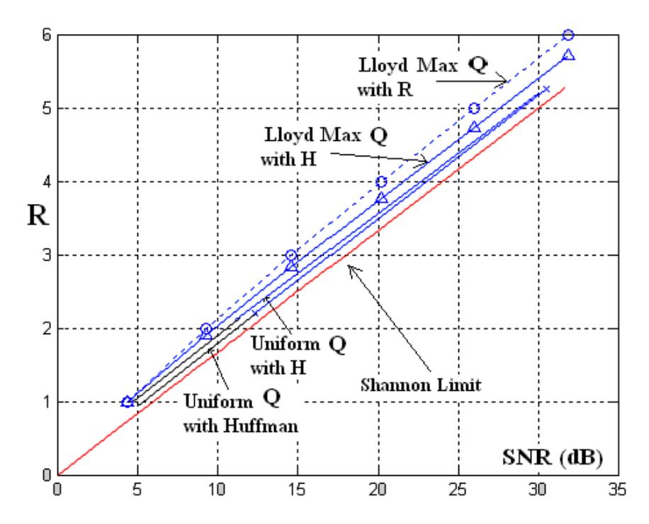
Figure 17 The performance of Non-Uniform (Lloyd Max) and Uniform Quantiser Against its Shannon Limit (Q stands for Quantisers).

As can be seen, the performance of uniform quantiser has successfully outperformed the non-uniform quantiser (Lloyd Max), as indicated by D and H which are closer to Shannon limit, compared to non-uniform quantiser.

4 Concluding Remarks

Experimental results indicate that in terms of signal to noise ratio, the uniform quantiser has successfully outperformed the performance of the non-uniform quantiser, as indicated by its closer rate in approaching the Shannon limit. Yet the performance improvements are more noticeable at higher bit rates rather than the lower ones.

In this research, Huffman coded uniform quantiser has successfully achieved reasonably close rate to Shannon limit. Subsequently, it is closely followed by entropy coded uniform quantiser H. In general, the uniform quantiser has demonstrated its superior performance compared to the non-uniform quantiser, represented by Lloyd Max.

Acknowledgements

The authors wish to thank Dr. Khee. K. Pang, a reader at the Department of Electrical and Computer Systems Engineering, Monash University, VIC, Australia for the completion of this research project.