
1 Introduction
In recent years, the transmission of multimedia content using mobile devices has become very popular. Teleconference, video streaming and digital television are just some examples of its applications. The demand for multimedia content via mobile devices is getting higher. This will invariably result in heavier demands on the radio spectrum and hence, air bandwidth will remain a bottleneck.
Uncompressed video data usually need considerable data storage capacity and data transmission bandwidth. Furthermore, uncompressed video data can influence transmission time needed. Large space requirement, high computational cost, and long transmission time are only some problems in transmitting video or multimedia content. For example, transmitting a 5 minute PAL video via a modem at 56 kilobits per second would take about 91.2 hours [1].
Despite the improvements made in media storage technology, compression techniques and the performance of transmission media, the demand for greater data storage capacity and faster transmission speed will continue to exceed the capabilities of current technologies. Furthermore, mobile computing device justifies research efforts into video compression research because unlike their desktop counterparts, internet access is badly affected by low air bandwidth.
There are several transformation techniques used for compression. The Discrete Cosine Transform (DCT) and the wavelet transform are two commonly preferred transforms to date. Previous works [2] showed that wavelet is better than DCT in its quality result [3]. The main concern of this paper is waveletbased video compression schemes for mobile devices like mobile phones and personal digital assistants (PDAs).
The remainder of this paper is organized as follows. Section 2 briefly discusses the basics of video compression and motion estimation. Section 3 presents two popular block matching algorithms and this is followed by an overview of the dual-tree complex wavelet transform in Section 4. Section 5 presents the hybrid proposed motion estimation. The results and discussion of the proposed algorithm are presented in Section 6. Finally, some conclusions are described in Section 7.
2 Video Compression and Motion Estimation
Prior to the advent of digital storage, video data are stored as analog signal on magnetic tape. In recent times, new digital technologies have emerged that enable users to store and view video digitally. However, video data, like other uncompressed multimedia data, usually require considerable data storage capacity and data transmission bandwidth. This can pose considerable problems for communication networks due to the potentially large volumes of data involved. One way to overcome this problem is by compressing the video data.
The main function of a video codec is to compress and decompress video and Figure 1 is a typical video codec.
The motion estimation of the current frame is computed with respect to a previous frame on the encoding side. From the blocks of image of the previous frame, a motion compensated image for the current can be formed. The output of the encoder side is the motion vectors for the blocks of images. Together with these motion vectors, the difference of the compensated image with the current frame is JPEG encoded and send to the decoder. The whole process is reversed and a full frame is formed on the decoder side. The underlying idea of motion estimation based video is to save on the number bits send. This is achieved by sending JPEG encoded difference images which can be highly compressed.
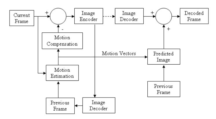
Figure 1 A Typical video codec [4].
Motion estimation is the process of finding the best match corresponding block to predict a new frame from the previous frame and it can improve compression ratios. This is achieved by compressing redundant information between successive frames. The rational for using motion estimation is that in a typical video sequence there are very few changes in conservative video frames. Changes are usually caused by sudden moments within a video frame. Motion estimation methods can be classified into several types. The three common types of motion estimation are block matching [5],[6] phase correlation [7]-[9], and gradient field correlation [10],[11]. Each of the methods has its own advantages and disadvantages. Block based methods have been widely used in many applications in motion estimation and can be implemented without much difficulty as compared to other methods. Gradient field [12] and phase correlation method [13] are promising methods but they require a lot of effort to calculate the gradient field and or phase information of signal respectively.
3 Block Matching Algorithm
Block matching techniques are popular and efficient motion estimation techniques and have been used in various standards, ranging from MPEG1/ H.261 to MPEG4/H.263. This section will briefly review two existing block matching algorithms. The following section will look at the basics of block matching.
3.1 Block Matching Basics
The current frame of a video can be divided into a matrix of macro blocks. These macro blocks are then compared with corresponding blocks and its adjacent neighbors in the previous frame. This is done so that a vector is generated to manage the movement of a macro block from one location to another. Using 'p' pixels of all four sides of the corresponding macro block from the previous frame the search area can be computed and 'p' is known as the search parameter [14]. This is illustrated in Figure 2. If the value of 'p' is large then the motions will be large. As a consequence the search parameter will be larger. This in turn makes the computation of the motion estimation computationally expensive.
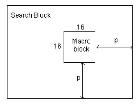
Figure 2 Block matching a macro block [14].
The least cost is achieved when one of the macro blocks makes a near perfect match with the current block. There are different cost functions and one popular cost function is the Mean Absolute Difference (MAD) [4], which is given by Eq. (1).
\[MAD = \frac{1}{N^2} \sum_{i=0}^{N-1} \sum_{j=0}^{N-1} \left| C_{ij} - R_{ij} \right|\] (1)
In Eq. (1), N is the side of the macro bock. \(C_{ij}\) is the value of block C in row i and column j and \(R_{ij}\) is the value of block R in row i and column j. These two pixels are compared in the current macro block and reference macro block, respectively.
The MAD is a criterion used to determine which block should be used. Typically, the lower the MAD the better the match and block with the minimum MAD is chosen.
3.2 Diamond Search
One popular block matching algorithm is the Diamond Search (DS) and many variants of DS have been proposed. DS uses two different types of fixed patterns, one is the Large Diamond Search Pattern (LDSP) and another is Small Diamond Search Pattern (SDSP). The LDSP with nine search points is shown in Figure 3(a) and the SDSP with five search points is shown in Figure 3(b). These search patterns exploit the characteristic of the center-biased motion vector (MV) distribution of a video sequence.
Figure 3 (a) LDSP (b) SDSP.
At the beginning of the search process, the LDSP starts at the centre of the search window and this search is repeated until the minimal matching error (MME) is produced. When the size of fixed search pattern does not match the size of the actual motion, an over search or an under search will occur. This can cause certain search to be deficient and inaccurate. When a point that has the least weight assumes the position of origin for the following search steps, then the search pattern is switched to SDSP. The procedure keeps on doing SDSP until least weighted point is found to be at the center of the SDSP.
In addition, LDSP can be too small for searching large MV and as a result it directs to either a long search path or being trapped into a local minimum matching error point. This can cause unnecessary intermediate searches and yields large matching errors. Consequently, the quality of the video is poor. On the other hand, it has less adaptability and search efficiency in tracking large motions 15.
3.3 Adaptive Rood Pattern Search
Another popular block matching algorithm is the Adaptive Rood Pattern Search (ARPS). ARPS consists of two stages, that is, an initial search and a refined local search. The initial search is carried out only once for each macro block to determine a suitable starting point, which is then used in the refined local search. This reduces the number of unnecessary intermediate search. The ARPS
algorithm makes use of the available MV of the neighboring MBs to determine the ARP size. An example is shown in Figure 4.
Figure 4 Adaptive Rood Pattern Search [14].
The four vertex points are placed equal distance with reference to the center point. The algorithm checks the location pointed by the predicted motion vector. In addition, it also checks the rood pattern distributed points, that is, the four vertex points. This rood pattern search puts the search in an area where there is a high probability of finding a good matching block. This effectively reduces unnecessary intermediate searches. A further small improvement in the algorithm is made by including the Zero Motion Prejudgment (ZMP), resulting in an algorithm called ARPS–ZMP, which helps to reduce the computational cost [15].
The correlation between the current block and the adjacent blocks in the spatial and or temporal domain can be used to predict the motion vectors (MV). The statistical average of neighboring MVs can be utilized to derive the predicted MV. The size of the search window can than be identified and used to perform the full search. With this method a good performance can be achieved at the prediction computational cost [15]. Each pattern of block matching algorithms achieves different transaction between algorithm complexity, search speed and picture quality. The results indicate that inter block correlations dynamically determine the size of the search pattern.
When compared with DS, ARPS–ZMP significantly increases the computational gain with little reduction in average PSNR. In addition, ARPS– ZMP improves average PSNR performance in large motion video sequences15. Therefore, this paper concluded that ARPS is a very efficient and robust motion estimation algorithm for real-time video coding applications. Usually, ARPS is occupied with Discrete Cosine Transform (DCT), but in this paper, combination with wavelet will be presented.
4 Dual Tree Complex Wavelet Transform
One of the key components in a video compression algorithm is the transform. As one of the main concerns of this work is video compression this section will therefore, discuss the relevant transform used, which is the discrete wavelet transform (DWT). DWT was developed to circumvent the problem of heavy computation load encountered in continuous wavelet transform. The standard DWT is a powerful tool, but has the following disadvantages, and these are shift variance, poor directionality, and absence of phase information. These disadvantages weaken DWT application for certain signal and image processing tasks [16].
The results of DWTs are real valued transform coefficients with limitations mentioned earlier. Fortunately, there are ways of reducing these limitations with a limited redundant representation in complex domain. The use of complexvalued 'analytic filters' can help to resolve the phase information, and shiftsensitivity problems experience with DWTs. These approaches are commonly referred to as 'Complex Wavelet Transforms' (CWT). CWTs can be broadly divided in two groups, that is, Redundant CWTs (RCWT) and Non-redundant CWTs (NRCWT). The RCWT groups include two almost similar versions of CWTs and they are Kingsbury's dual-tree complex wavelet transform (DTCWT) [23]-[26], and Selesnick's DTCWT [17].
As mentioned in the above discussion, one the limitation of DWT is the lack of shift invariance, which is a result of down-sampling in the DWT. In downsampling every alternate wavelet coefficient is discarded. As a result the wavelet coefficients are location sensitive in the sub-sampling pattern. What this means is that a small shift in the input waveform can cause large changes in the wavelet coefficients. If there large changes in wavelet coefficient then this could lead to large changes in the reconstructed waveforms.
The DWT lack of shift invariance means that DWT cannot be directly used for motion estimation. However, there exists a solution that can overcome the shift invariance. One way to minimize shift variance is to construct two wavelet decomposition trees, one for a mother wavelet with even symmetry and the other for the same mother wavelet, but with odd symmetry [18]. This is illustrated in Figure 5. Wu et al cited that the DTCWT has limited redundancy as compared to the real DWT. In addition, Wu et al also cited that the DTCWT has approximate shift invariant, improved orientation selectivity and perfect reconstruction [19].
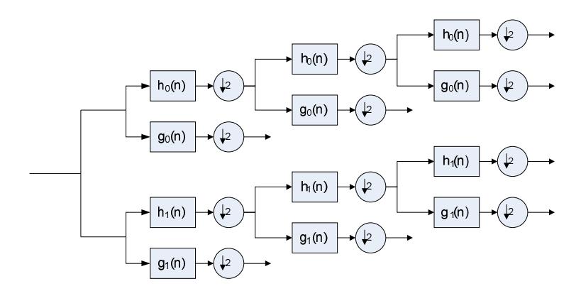
Figure 5 Three level DTCWT [26].
The DTCWT implements the complex transform of a signal using two separate DWT decompositions as shown Figure 5. The filters banks (FBs) are designed in such a way that the upper FB yields the real part of the complex wavelet transform, and the lower FB yields the imaginary part. The upper FBs are lowpass/ high-pass filters (h0(n), h1(n)) and the lower FBs are low-pass/high-pass filters (g0(n), g1(n)) and they are designed so that the complex wavelet ψ(t) := ψh(t) + jψg(t) is approximately analytic and also that ψg(t) is approximately the Hilbert transform of ψh(t)[26].
The advantage of the DTCWT is that it provides a high degree of shiftinvariance in its magnitude but it is computationally expensive. For example, applying the DWT to an n-by-n image, the result would be n-by-n values. However, using the DTCWT, the result would be 4 n-by-n values. So, in other words the result is four-time redundancy but the upside is that there is a high degree of shift-invariance in magnitude. This is a reasonable tradeoff for applications that need a high degree of shift-invariant.
5 Proposed Algorithm
This section will give an overview of the proposed motion estimation algorithm. The algorithm is a combination of DTCWT combined with ARPS where usually ARPS is combined with DCT. ARPS is used because it takes up less computational time than other block matching algorithms. The reason for utilizing the DTCWT is that it has a shift invariant property, which is useful in motion estimation [20] as discussed earlier. It is envisaged that the combination of ARPS and DTCWT can improve PSNR result [21].
The new proposed algorithm is as follows:
- Step 1: Perform DTCWT decomposition. For each video frame, the DTCWT is performed to obtain the scale and wavelet coefficients.
- Step 2:Estimate the wavelet coefficients of the current frame n+2 with DTCWT to compute motion vector.
- Step 3: Carry out ARPS algorithm motion estimation[4].
o Perform SDSP
 1. Initialized the index points for SDSP
 2. Set check matrix to zero
 3. Start SDSP
      3.1 Keep track of no. of blocks evaluated
      3.2 Scan image starting from top left of image
      3.3 Set corresponding element in matrix to 1 after
      point is checked.
      if in left most column
      step size = 2;
      else
      Re-compute step size
      if
      motion vector is one of the LDSP points
      check the rood pattern 5 points
      else
      check 6 points
      3.4 Repeat until scan is complete
  o Step 3.2 Perform LDSP
     1. Initialize the index points for LDSP
     2. Start SDSP
      2.1 Scan image
      2.1.1 Compute row/vertical co-ordinate for
     ref block
      2.2.2 Compute col/horizontal co-ordinate for
      ref block
      if vertical block > row and horizontal
      block > col
      continue outside image boundary
      end
      if
      center point is calculated
      end
     2.2 Set corresponding element in matrix to 1 after
     point is checked.
      2.3 Repeat scan is complete
Step 4: Perform motion compensation[4].
end
- 1. Scan starts at top let side of image
- 2. Scan in steps for every macro-block for motion vectors
- 3. Place the macro-block from the reference image onto the compensated image
- 4. Repeat step 2 and 3 until scan is complete
- Step 5: Reconstruct the motion-compensated image is obtained via the inverse transform.
Motion in each sequence is also considered when grouping these data. They are grouped into five groups as presented in Table 1.
| Group | Sequences | Moving Area (%) | ||
|---|---|---|---|---|
| 1 | Hanif | 84.13 | ||
| 2 | Missa | 84.70 | ||
| 3 | Susie | 85.87 | ||
| 4 | Caltrain | 91.64 | ||
| 5 | Football | 94.99 | ||
Table 1 Moving Area.
As shown in Table 1, groups of video are sorted ascending based on percentage of moving area and background complexity. Nie and Ma use static area to show that a large percentage of zero-motion blocks are encountered in such type of video sequences. In this paper, moving area is determined by subtracting each frame with the next frame. This research tested sequences, each has 32 frames. Its non-zero difference between frames that represents their motion is then compared with whole area of frame.
moving area(%) = \[\frac{amount of \ non \ zero \left\{frame (n) - frame (n+1)\right\}}{frame \ size} x 100\%\]
Figure 6 shows the movements of Hanif sequence. The figure shows the element difference between Hanif frame 001 and frame 002. Black area indicates static area while the moving area is in white.
Figure 6 Hanif Sequences.
It can be seen that movement is concentrated on Hanif himself and ball. The white areas showed a little shifted movement because non static camera has been used to do the recording.
Figure 7 Missa Sequences.
The Missa video sequence resembles a newsreader. In the video sequence, Missa moves her head and which in turn influences her shoulders movement. Meanwhile background is static. The color brightness of her clothes is similar to the background. All these factors consider she looks static even actually there are few movements. Difference of Missa frame 001 and frame 002 is taken to be shown in Figure 7. White area of Missa is spread out. It seems so wide but in fact, most of those are not movements.
Figure 8 Susie Sequences.
The Susie video sequence is similar to the Missa video sequence. The difference is that the Susie video sequence focuses on facial movement. The Susie video sequence is shown in Figure 8. White area, which represents the moving part, covers most parts of each frame and notes the difference between frame 001 and frame 002.
Figure 9 Caltrain Sequences.
The Caltrain sequence in next group has two kinds of motion. First is the movement of the mobile and the second is the movement in the background. Figure 9 shows that mobile is moving to the left and the background is shifted to the right as long as the camera tracks the movement of the train.
Figure 10 Football Sequences.
The Football sequence is a representation of complex motion sequences. It can be seen that there is a lot of movement. This is a big contrast to the previous video sequences presented. The Football video sequence can be seen in Figure 10.
As shown in Figure 10, the area with white color indicates moving area while the areas that are black are the static area. If the whole part of this sequence is viewed, it can be seen that the direction of their motions is spread out and random.
6 Results and Discussion
The following is a discussion of the results obtained using the proposed algorithm presented earlier. The following section will include a discussion of the advantages of this proposed algorithm for video compression for mobile devices.
| Sequences | Method | Computation Cost | Execution Time (s) | PSNR (dB) |
|---|---|---|---|---|
| Football | DCT + ARPS | 10.724 | 8.3044 | 20.577 |
| DTCWT + ARPS | 10.708 | 8.2870 | 21.810 | |
| Caltrain | DCT + ARPS | 9.763 | 8.352 | 21.163 |
| DTCWT + ARPS | 10.071 | 8.8 | 23.149 | |
| Hanif | DCT + ARPS | 6.8113 | 7.1949 | 31.610 |
| DTCWT + ARPS | 6.8963 | 7.5757 | 31.977 | |
| DCT + ARPS | 7.3283 | 7.2744 | 34.187 | |
| Missa | DTCWT + ARPS | 8.6490 | 8.0243 | 36.164 |
| Susie | DCT + ARPS | 5.903 | 6.2504 | 34.069 |
| DTCWT + ARPS | 5.8121 | 6.0843 | 38.674 |
Table 2 Comparison of Sequences.
As mentioned earlier, computational cost is one of problems in compression. It is also related with time needed. Computational cost will be higher when a more complex algorithm is executed. In this paper, computation is computed based on how many times Mean Absolute Difference (MAD) has been executed divided by the amount of blocks that have been evaluated [4].
With reference to Table 2 it can be seen that for most sequences, the hybrid method yields better PSNR value but requires more computation and time (except for Football and Susie sequence). Time is an important parameter for comparing several algorithms in video processing.
By applying the DTCWT to an n-by-n image, the result would be 4 n-by-n values. So, in other words the result is four-time redundancy but since that there is a high degree of shift-invariance in magnitude. This is a reasonable tradeoff for applications that need a high degree of shift-invariant. That is why in Missa, Caltrain and Hanif sequences, it is shown that the computations and time needed increases linearly. In Susie and Football sequences, there is a lot of shifted motions so computations as well as time consuming are decreased.
In summary it observed that as computational cost increases, more execution time also increases. On the other hand, execution time and computational cost decrease when there is a lot of shifted motions like in Football sequence.
6.1 Memory Usage
Mobile devices have limited memory but the video codec algorithm requires significant memory resources. The comparison of memory usage for several video sequences is shown in Table 3.
| Sequences | Method | Memory Usage (kB) | Mem Usg (kB) |
|---|---|---|---|
| Susie | DCT + ARPS | 2965 | 47 |
| DTCWT + ARPS | 2928 | ||
| Hanif | DCT + ARPS | 828 | 60 |
| DTCWT + ARPS | 768 | ||
| Caltrain | DCT + ARPS | 2387.4 | |
| DTCWT + ARPS | 2236 | 151.4 | |
| Missa | DCT + ARPS | 1428 | |
| DTCWT + ARPS | 1212 | 216 | |
| Football | DCT + ARPS | 3780 | |
| DTCWT + ARPS | 2882.4 | 897.6 |
Table 3 Memory Usage of Video Sequences.
As it can be seen from the results in Table 3, the difference of memory usage varies. For Missa sequences, the memory usage is 216 kB, while for Hanif sequence the memory usage is 60 kB respectively.
The maximum difference is reached by Football sequence. It shows that complexity in motion is not a guarantee for decreasing of memory usage while it still requires large enough memory to execute the algorithm.
6.2 Visual Quality
In order to ascertain the subjective visual quality based on human perception, a survey was carried out with some undergraduate students. This group of students was chosen because they are mobile telephone users or potential mobile telephone users who are most likely to use stream video using mobile telephones. Each student was asked to rate each image based on the following values.
Value Rating Description 1 Excellent An extremely high quality video. 2 Fine A high quality video. Artifacts are not objectionable. 3 Passable An acceptable quality video. Artefacts are not objectionable. 4 Marginal A poor quality video. Artefacts are somewhat objectionable. 5 Inferior A very poor video, but still acceptable. Artefacts are visible and objectionable. 6 Unusable A bad video that it is unacceptable.
Table 4 Visual Quality Evaluation.
The above rating scheme is a modified version of Frendendall and Behrend (1960) work for evaluating television images. The modified version [22] was used to evaluate compressed still images.
Sequence A is using ARPS only meanwhile B is using the proposed algorithm. The results are shown in the following figures.
For Hanif sequence, it can be seen in Figure 11 that Hanif A is passable (3) and Hanif B is fine (2). For Hanif A, the values are concentrated in passable (3) and marginal (4) meanwhile for Hanif B, it ranges from excellent (1) to marginal (4). These results implied that the proposed hybrid algorithm can perform better than the ARPS.
For Susie B, most respondents award a fine (2) and marginal (4) for Susie A. It shows that the proposed method is comparable with the original ARPS method. It also indicates that the proposed method can work better for sequence whose motion is not so complex but the moving area is quite wide.
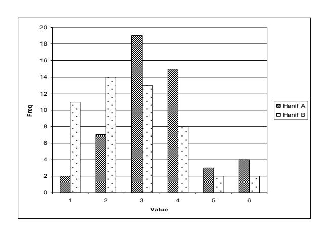
Figure 11 Subjective Visual Quality of Hanif Sequence.
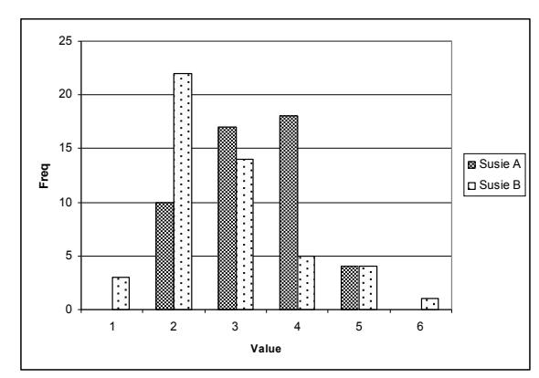
Figure 12 Subjective Visual Quality of Susie Sequence.
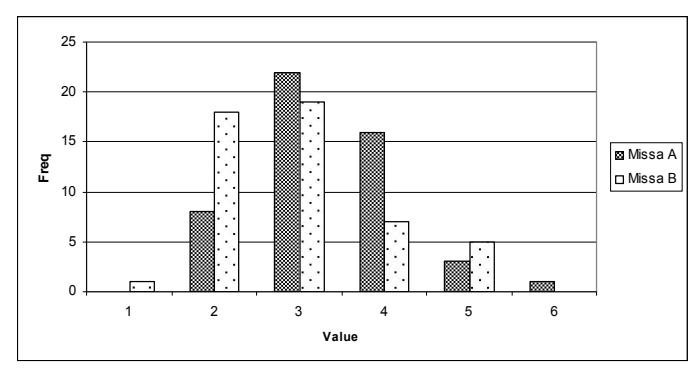
Figure 13 Subjective Visual Quality of Missa Sequence.
The majority responders put Missa A and B on passable (3) as shown in Figure 13. But it can be seen that for Missa B, the value is between fine (2) and passable (3) while for Missa A is around passable (3) and marginal (4). It means that the proposed method still can perform better against the DCT based method. In this group, the sequence does not have complex motion. Respondents can easily see the picture in every frame.
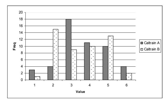
Figure 14 Subjective Visual Quality of Caltrain Sequence.
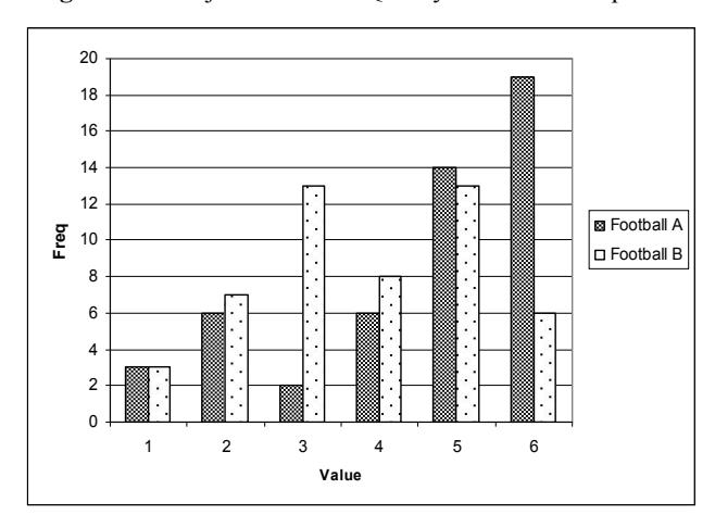
Figure 15 Subjective Visual Quality of Football Sequence.
Most respondents give a Passable (3) for Caltrain A and fine (2) for Caltrain B as shown in Figure 14. This respond suggests that the proposed method result is still comparable with DCT based methods. It shows that even for rather complex motion, the proposed method has good potential.
For Football A sequence, most respondents have chosen this as the worst quality, unusable (6). Meanwhile, most respondents agreed that the quality of Football B is passable (3) as can be seen in Figure 15. Many respondents reported that they have problem viewing it clearly because of its complex motion.
DTCWT-based DCT-based
Figure 16 Visual Results.
Figure 16 is the final result of both methods. It should be noted, at first glance there seems to be no difference between them. But the PSNR measurement and subjective visual quality assessment indicate that DTCWT-based algorithm is better than DCT-based algorithm.
7 Conclusion
In this paper a hybrid motion estimation algorithm utilizing the Dual Tree Complex Wavelet Transform (DTCWT) and the Adaptive Rood Pattern Search (ARPS) block is presented. The paper began with a discussion of video compression and motion estimation, block matching algorithm, and DTCWT. A visual quality scoring system shows that potential gains can be achieved from the new proposed algorithm. The preliminary results also show that the PSNR and visual quality is improved and less memory is required for the algorithm.
One possible direction for future work is to consider a hardware implementation of a wavelet-based motion estimation for a video codec, which can be incorporated into a mobile device. A special purpose FPGA chip may be designed and fabricated to implement the algorithm. This would significantly improve the video codec performance.
In conclusion, this paper has demonstrated that a wavelet-based and ARPS algorithm approach to motion estimation can offer improvements in video compression for mobile applications.