
1 Introduction
Elliptic Curve Cryptography (ECC) is a public-key encryption that requires high computation for solving complex arithmetic operations. Elliptic curve is used in cryptography because of its special mathematical properties match cryptographic requirements for encryption and decryption. Elliptic curve has its own arithmetic operation, that is very specific and unpredictable, makes it cryptographically strong and becomes the most preferable cryptography algorithm to replace RSA. Unfortunately, implementing ECC requires sophisticated mathematical skills. There are many layers, restrictions, and combinations that make various ECC implementations difficult to compare. Every level of ECC offers many things to explore. In this work we focus on the lowest level: finite field operations. Since multiplication is the most frequently used operations, we investigate existing multipliers algorithms and make improvements.
The keylength used in ECC determines the level of security. In general, longer key requires more components in the corresponding hardware implementation. As the internet technology grows, the demand to implement ECC on constraint devices increases. As a consequence, there is a need for efficient algorithm and architecture for implementing ECC on constraint devices. To fulfill the security level requirement at the present, ECC should have above 160 bits keylength.
We choose to implement 299 bits in this research. However implementing 299-bit ECC in constrained devices, simulated with FPGA board, cannot be done using conventional algorithm and architecture. For example, 299-bit binary classic multiplier cannot fit in most FPGA devices. One alternative solution is by using composite field.
Composite field can be seen as a finite field divided into subfields (ground fields) and extended fields. The representation of composite field can be seen as composing a long string of bits into smaller groups of bits. This representation allows arithmetic operations to be done in smaller chunks of string so the complex operations can be broke down into simpler operations. The focus of our paper is the implementation of multiplier using composite field. We focus on multiplier because multiplication is the most frequently used operation in ECC. The benefit of using composite field is the lower of memory usage and lower components. Thus if the process of multiplication is more efficient, the whole performance of cryptosystem will be improved.
This work uses of composite field characteristic of dividing one big chunk of operation into smaller ones, with the classic multiplication for the extension field multiplication and LUT for base multiplication. We chose to use the easiest multiplier algorithm just to confirm the idea that composite field is promising to be able to perform operations for long bits.
2 Background and Previous Work
2.1 Elliptic Curves
Given a field F of characteristic 2, an elliptic curve E over F is an equation of the form
\[v^2 + a_1 x v + a_2 v = x^3 + a_2 x^2 + a_4 x + a_6\] where \(a_1, a_2, a_3, a_4, a_6\) in F.
The set of rational points on E over F denoted by E(F) is
\[E(F) = \{(x,y) \in F^2 : y^2 + a_1xy + a_3y = x^3 + a_2x^2 + a_4x + a_6\} \cup \{0\}\] where O is the projective closure of the equation \(y^2 + a_1xy + a_3y = x^3 + a_2x^2 + a_4x + a_6\). The point O is called the point at infinity.
The set of rational points E(F) carries a commutative group structure with some addition operation with the point at infinity acting as the zero element. The following is the explicit formula for the group operation.
Composition Rule. Let \(P,Q \in E\), and L be a line connecting P and Q (the tangent line of E if P = Q), and R the third point which is the intersection of L and E. Let L' be the line connecting R and Q. Then P + Q will be the point where L' intersect E.
Proposition 1. The composition rule above satisfies the following:
If L intersect E at P,Q,R (not necessarily different) then (P+Q)+R=O.
- 1. P+O=P for all \(P \in E\)
- 2. P+Q=Q+P for all \(P,Q \in E\)
- 3. For all \(P \in E\) there exists a point (-P), such that P+(-P)=O
- 4. For all \(P, Q, R \in E(P+Q) + R = P + (Q+R)\).
- 5. Hence E with the composition rule form an abelian group with identity O.
Explicit Group Operation. Let E be an elliptic curve satisfies the Weierstrass equation
\[E: y^2 + a_1xy + a_3y = x^3 + a_2x^2 + a_4x + a_6\]
- 1. Let \(P_0 = (x_0, y_0) \in E\). Then \(-P_0 = (x_0, -y_0 a_1x_0 a_3)\).
- 2. Let \(P_1 + P_2 = P_3\) with \(P_i = (x_i, y_i) \in E\). If \(x_1 = x_2\) and \(y_1 + y_2 + a_1x_2 + a_3 = 0\), then \(P_1 + P_2 = O\).
Otherwise, let
\[\mu = \frac{y_2 - y_1}{x_2 - x_1},\] \[\vartheta = \frac{y_1 x_2 - y_2 x_1}{x_2 - x_1}\] for \(x_1 \neq x_2\), and \[\mu = \frac{3 x_1^2 + 2a_2 x_1 + a_4 - a_1 y_1}{2y_1 + a_3 + a_1 x_1}\] \[\vartheta = \frac{-x_1^3 + a_4 x_1 + 2a_6 - a_3 y_1}{2y_1 + a_3 + a_1 x_1}\] for = .
Then = + is the line through P1and P2, or the tangent line of E if P1= P2.
3. P3 = P1 + P2 is given by
\[x_3 = \mu^2 + a_1 \mu - a_2 - x_1 - x_2\]
\(y_3 = -(\mu + a_1)x_3 - \vartheta - a3.\)
For an integer m and P∈ E, define
\[[m]P = P + ... + P (m \text{ terms}) \text{ for } m > 0,\]
\([0]P = O, \text{ and } [m]P = [-m](-P) \text{ for } m < 0\)
The El Gamal elliptic curve encryption based on binary field is as following:
INPUT: Elliptic curve domain parameter (k,E,P,n), public key Q, plaintext m
OUTPUT: Ciphertext (C1,C2)
- 1. Represent the message m as a point M in E(GF(2k ))
- 2. Select k ∈[1, n-1]
- 3. Compute C1=[k]P
- 4. Compute C2=M+ [k]Q
- 5. Return (C1,C2)
The encryption process is shown in Figure 1
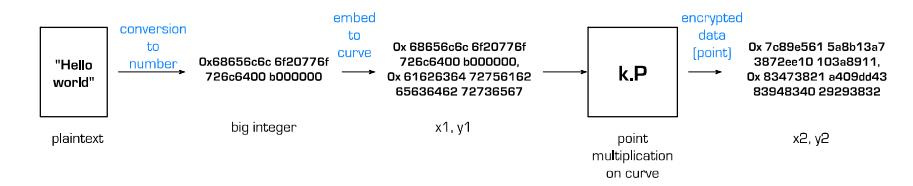
Figure 1 Encryption process in ECC.
For the decryption is as following:
INPUT: Elliptic curve domain parameter (k,E,P,n), private key d, ciphertext (C1,C2)
OUTPUT: Plaintext m
- 1. Compute M= C2 –[d] C1
- 2. Extract m from M
- 3. Return (m)
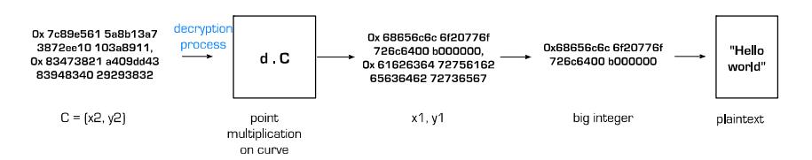
Figure 2 Decryption process in ECC.
From the elliptic curve encryption and decryption and elliptic curve operation, one can see that the role of operations in ground field is very important. In this research we choose composite field as the ground field.
2.2 Composite Fields
Assume that is a number to be used to construct a field.does not have to be prime if the order of the finite field is power of a prime or = where is a prime. Thus the finite field can be extends to an extension field so the field () can be extended to (()).
Both in hardware or software implementation performing finite field arithmetics, choosing q=2 is a big advantage because information is only representated in 0 or 1.
Referring to [1], certain kinds of finite field can be defined as:
Two pairs of \(\{GF(2^n)\}\), \(Q(y) = y^n + \sum_{i=0}^{n-1} q_i y^i\) dan \(\{GF((2^n)^m)\}\), \(P(x) = x^m + \sum_{i=0}^{m-1} p_i x^i\) is a composite field if \(GF(2^n)\) is constructed as extension field of GF(2) by Q(y) and \(GF((2^n)^m)\) is constructed as extension field of \(GF(2^n)\) by P(x). Q(y) and P(x) is irreducible polynomials over GF(2).
Mathematically, \(GF((2^n)^m)\) is isomorphic to \(GF(2^k)\) for n.m = k [2]. Although a field of order \(2^{nm}\) is isomorphic to a field of order \(2^k\), the algorithmic complexity of both fields are different in additions and multiplication operations. Generally it depends on the chosen m and n and more specifics on polynomials Q(y) and P(x) [3].
All curve representations in \(GF(2^k)\) can be converted to curves in \(GF((2^n)^m)\). If both F and F' are finite fields with equal number of elements, there exists way to correlate each element in F with corresponding element in F' so addition and multiplication tables of F and F' are equal (F and F' isomorphic)[4], Theorem 2.60 page 104.Curve representations in composite field converted to noncomposite field has been done in [5].
In finite field, composite field can perform same operations as non-composite. Only the operation has to be modified to be able to do in composite representation. In composite field, the field is divided into sub-fields. \(GF(2^8)\) can be divided into \(GF((2^2)^4)\) or \(GF((2^4)^2)\). Sub-fields can be processed faster dan implemented in parallel.
The reason why we use \(GF((2^{13})^{23})\) in this implementation is because \(GF((2^{13})^{23})=GF(2^{299})\) which complies with the security level needed. The other reasons is that GCD(13,23)=1 so irreducible polynomial can be used for both ground field and extension field, and there are trinomials and polynomials available. Carefully chosen irreducible polynomial will reduce the complexity of multiplication operation.
Previous Works. The first idea multiplier for composite field was initiated by Mastrovito [6]. The multiplier is called hybrid-multiplier. It performs the multiplication by doing multiplication serially in the ground field and parallel in the extension field. Mastrovito's multiplier basically works using a multiplication matrix that includes the reduction process. Paar in his works [3],[7],[8] added some improvements to Mastrovito's. Paar implemented
multiplication in the ground field using KOA and Mastrovito for multiplication in the extension field. Later, Rosner [9] conducted further research of Mastrovito and Paar.
Look-Up Table (LUT) for composite field operations has been implemented in [9]. The algorithm for ground field multiplication using logaritmic table lookup is proven to be fast.
3 Methodology
3.1 Look-Up Table (LUT)
LUT is used for storing log and alog (anti log) table to make multiplication operation in the ground field \(GF(2^n)\) perform faster. In [2] it is concluded that n does not have to be exactly the same as a single computer word (e.g. 8, 16). It has been proved that n < 2 is more efficient because the table will be smaller and thus will take advantage of the first level cache of computers.
One of the reason why this research uses LUT for storing precomputed log and alog table in \(GF(2^{I3})\) is that Table 2 in [2] shows that LUT for n=13 is efficient for polynomial basis multiplication compared to bigger n. To construct logaritmic lookup table, a primitive element g in \(GF(2^n)\) is selected to be the generator of the field \(GF(2^n)\), so that every element A in this field can be written as a power of g as \(A=g^i\), where \(0 \le i \le 2^n-1\). Then the powers of the primitive element \(g^i\) can be computed for \(i=0, 1, 2, \ldots, 2^n-1\), and obtain \(2^n\) pairs of the form (A, i). Two tables sorting these pairs have to be constructed in two different ways: the log table sorted with respect to A and the alog table sorted with the respect i. These tables then can be used for performing the field multiplication, squaring and inversion operations. Given two elements A, B in \(GF(2^n)\), the multiplication C=AB is performed as follows:
1. i := log[A]
2. \[j := log/B\]
3. \[k := i+j \pmod{2^n-1}\]
4. \[C := alog[k]\]
The steps above is based on the fact that \(C = AB = g^i g j = g^{i+j \mod 2n-l}\). Ground field multiplication requires three memory access and a single addition operation with modulus \(2^n-l\).
Savas and Koc [2] also proposed the use of the extended alog table for eliminating modular addition operation (step 3). The extended alog table is \(2^{n+l}\)-l long, which is about twice the length of the standard alog table. It contains the values \((k, g^k)\) sorted with repect to the index k, where \(k = 0, 1, 2, \ldots, 2^{n+l}-2\). Since the values of i and j in step 1 and 2 of the multiplications are in the range \(0, 2^n-l\), the range of k = i + j is \(0, 2^{n+l}-2\). Thus modular addition operation can be omitted and the ground field multiplication operation can be simplified as follows:
- 1. i := log[A]
- 2. j := log/B
- 3. k := i + j
- 4. C := extended-alog[k]
Figure 3 shows the process of reading LUT to compute multiplication using log and alog table.
Figure 3 Multiplying using LUT.
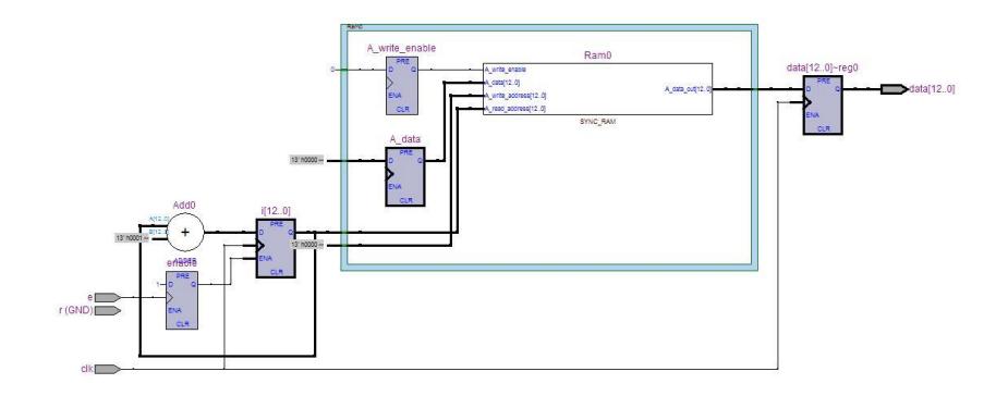
Figure 4 13-bit LUT implementation.
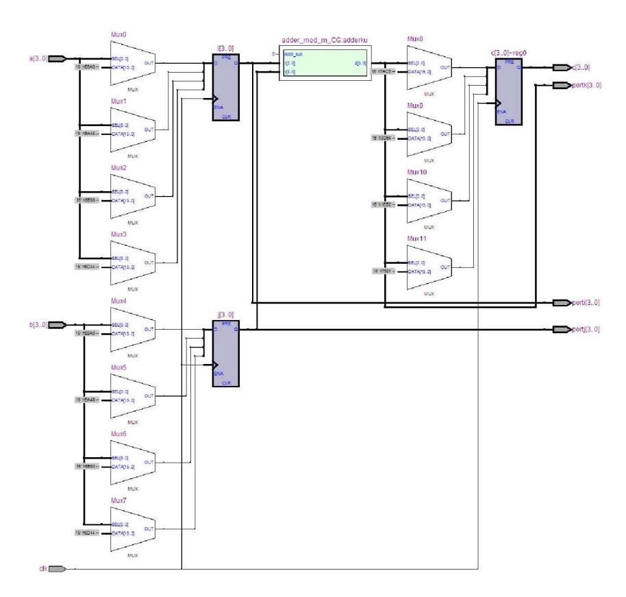
Figure 5 Multiplication of GF(24 ) using log and alog table with LUT.
Figure 6 The waveform of multiplication of \(GF(2^4)\) using log and alog table with LUT.
Figure 4 shows the RTL diagram of LUT implemented using Quartus and Altera DE2while Figure 5 shows the RTL of \(GF(2^4)\) using LUT for storing log and a-log table with algorithm from [2]. There are two LUTs in the implementation, one is for storing \(2^4\)-blocks log table, and the other is for storing \(2^4\) -blocks alog table. Log table put n-bits i values on the first column and n-bits \(g^i\) values on the second column. alog table sorted the table based on \(g^i\) values, and put the corresponding i values on the second column. Thus, each multiplier unit requires at least one LUT for storing i and j values in serial implementation and two LUTs for parallel implementation. Another LUT is needed for storing alog table.
Figure 6 shows the simulation waveform of multiplier implemented in Figure 5. As a comparison, Figure 7 shows that straightforward 299-bit implementation failed for the available resources.
4 Design and Implementation
The generic architecture of our circuit is shown in the Figure 8. On the left side there are two set of input registers, each for input A and B. The size of the input registers depends on the bit size. For our particular case, which is a custom design, it is 13-bit. If we use off the shelf components, we may have to use 16-bit registers since common components usually have \(2^n\) word size.
Figure 7 Failed implementation for straightforward 299-bit implementation.
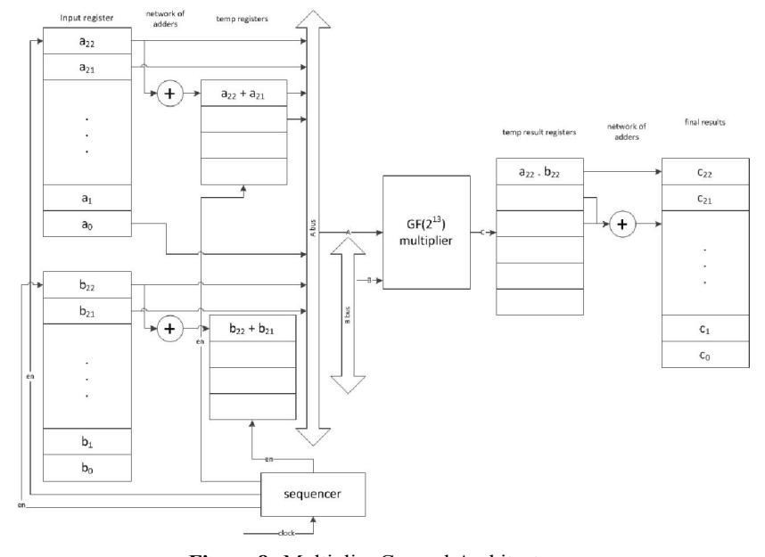
Figure 8 Multiplier General Architecture.
Right next to the input registers are temporary registers that are used to store addition terms before they are multiplied. The decision will effect the number of temporary registers (and adders needed).
In the center of our circuit is the GF(213) multiplier. In this particular design we have only one multiplier, implemented as LUT multiplier. Multiplication is done in serial fashion. Figure 9 shows an estimated timing diagram, which will be implemented in the sequencer. For example, when multiplying a22 andb22, the enable lines of registers related to those element and the result register are activated.
If area is permitting, we could add more multipliers to perform parallel multiplication. Additional multipliers will reduce the time to perform all multiplications at the expense of more area. Careful timing consideration must be done in order to avoid race condition is multiple multipliers are implemented.
The results of multiplications are stored in temporary registers before they are added to create the final results. Thus, there is a network of adders on the right side.
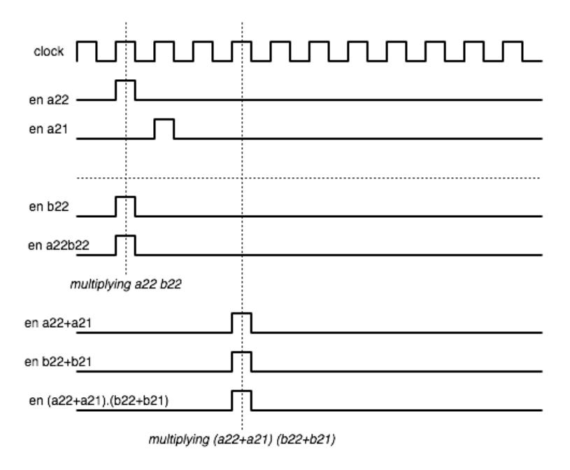
Figure 9 Estimated timing diagram.
Figure 10 below is the snippets of VHDL code LUT implementing GF(213) multiplier. A 13-bit multiplier requires 213entries ≈ 8000 entries, for each table. If we implement this in general purpose hardware then it should be implemented in 16 bit (2 bytes). In our implementation, the log and alog table occupies 2*8*2 bytes = 32 Kbytes .
process (clk) begin
if clk'event and clk = '1' then
case a is
when "0000000000000" => i <= "0000000000001";
when "0000000000001" => i <= "0000000000010";
when "0000000000010" => i <= "0000000000100";
when "0000000000011" => i <= "0000000001000";
when "0000000000100" => i <= "0000000010000";
when "0000000000101" => i <= "0000000100000";
…
Figure 10 Snippet ofGF(213) LUT implementation in VHDL.
ECC Processor Architecture. Figure 11 shows the general architecture of ECC processor. FFAU (Finite Field Arithmetic Unit) is an arithmetic unit specifically used for calculating finite fields operations.
The processor will accept input data (plaintext) through data_in pin then will process the command given according to the opcode. The processor will execute the command after "start" command. Status of the processor (busy, done) can be monitored through "status" line. After the process is done, the result (ciphertext) will be send through "data_out" pin. "reset" pin is used to return the processor to the initial state.
The ECC processor can process data in different length of bits. For long bits, the transfer process has to be carefuly considered to fit in the data bus. General
computers use 32-bits data bus. Meanwhile the data to be processed by ECC processor is more than 100bits length.
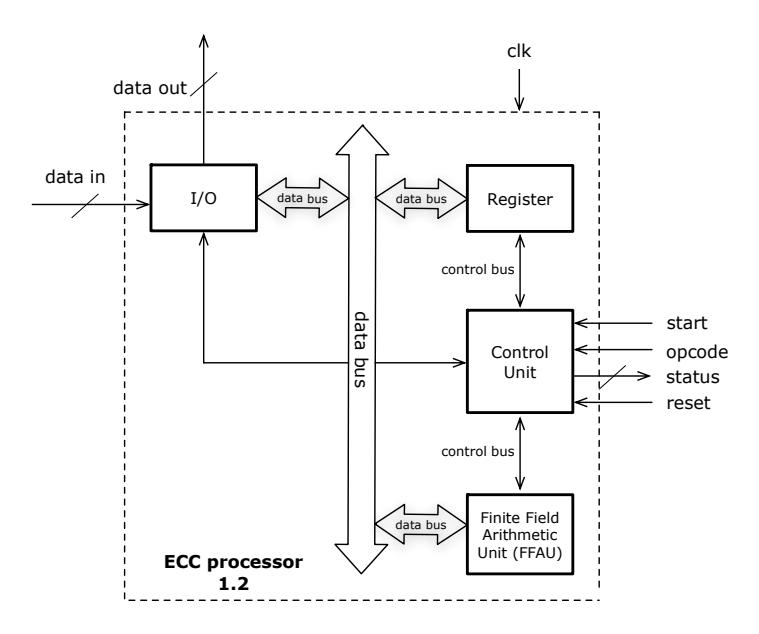
Figure 11 ECC top level processor architecture.
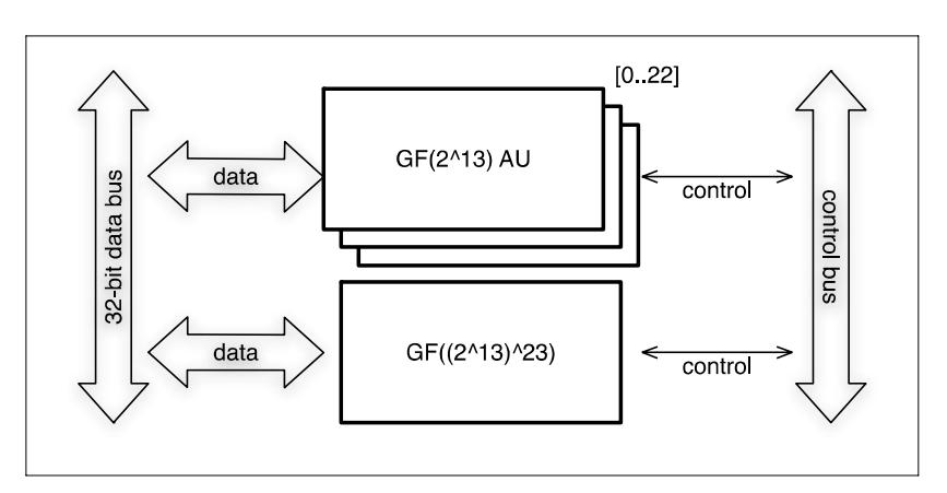
Figure 12 FFAU (Finite Field Arithmetic Unit).
One method to solve this is to divide data into several blocks (for example each blocks is 32-bit length) and load the data to the processor several times. Even for the most extreme cases, data can be loaded serially. This ECC processor has several parameters stored in the register. The parameters are elliptic curve equation used, private key and public key. The parameters can be stored permanently (hardcoded) or can be loaded through the "data_in" using a specific opcode. "reset" pin is used to set the parameter to the initial condition (for example all zero). At the earlier stage of research, the parameters are stored permanently to simplify the problem.
Figure 12 shows the block diagram of FFAU shown earlier in Figure 11. \(GF((2^{13})^{23})\) requires 23 \(GF(2^{13})\) multipliers. Figure 13 shows the concept of \(GF((2^{13})^{23})\) multiplier.
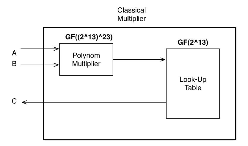
Figure 13 GF(2<sup>13</sup>)<sup>23</sup>) Classical Multiplier-LUT.
5 Analysis
We compare our composite field multiplier with standar non-composite multipliers: classic multiplier, interleaved multiplier, Karatsuba-Offman multiplier, Mastrovito multiplier Type-1 and Type-2 and Montgomery multiplier.
The experiment is done by running each multiplier using Quartus II Version 9.1 Build 350 03/24/2020 SP 2 SJ Web Edition. All multipliers are implemented using family device is Stratix II, device EP2S15F484C3.
As shown in Table 1, not all multipliers design fit in the standard device. Only interleaved multiplier and Mastrovito 2 multiplier can handle up to 233 bits.
Our design has been tested for lower bits and gives promising result that it can also works for 233 bits or more. This is the subject of our further research since the architecture should be customized to able to process longer bits.
Table 2 shows the result of all multipliers comparation based on logic utilization, combinational ALUT(s), dedicated logic registers, total registers and total pins. The performance of our multiplier is in general better than other multipliers except it requires more pins.
Our multiplier number of register is 56% lower than interleaved and Montgomery multiplier and 83% lower than Karatsuba multiplier. Karatsuba multiplier requires more register due to its recursive process in multiplying process.
The use of combinational ALUT is less than 1%, which makes our multiplier use combinational ALUT less than Mastrovito, Mastrovito 2, Classic and Karatsuba.
Our design uses more pins as a tradeoff of less registers and ALUT.
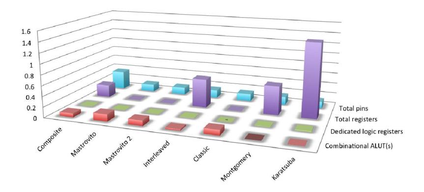
Figure 15shows gives multipliers compared with all variables. Figure 16 is the brief version of Figure 15, focusing on variables not significantly observed in Figure 15.
Multiplier Area Usage
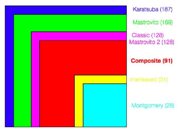
Figure 14 Multiplier Area Usage Comparison.
Combina-Dedica-Logic utiliza-Combina-Dedicated Total Total ted logic Total tional pins (%) Stratix II tional logic regis-ALUT(s) registers ALUT(s) tion (%) registers ters (%) (%) Composite Mastrovito 91/12480 24/12480 24 122/343 36 2 169/12480 0/12480 0 0 48/343 14 Mastrovito 2 2 128/12480 0/12480 0 0 48/343 14 31/12480 Interleaved < 1 55/12480 52/343 55 15 128/12480 28/12480 2 < 1 Classic Montgomery 0/12480 0 0 48/343 14 55/12480 55 52/343 15 < 1 187/12480 141/12480 44/343 Karatsuba
Table 1 Multiplier Comparison.
Table 2 Multiplier Processing Limit.
| Multiplier | m |
|---|---|
| Classic | 8, 16, 32, 64, 128, 163 |
| Interleaved | 8, 16, 32, 64, 128, 163, 233 |
| Mastrovito | 8, 16, 32, 64 |
| Mastrovito 2 | 8, 16, 32, 64, 128, 163, 233 |
| Montgomery | 8, 16, 32, 64, 128 |
| Karatsuba-Offman | 8, 16, 32, 64 |
| Composite | *our experiments so far shows |
| a strong indication that it is | |
| implementable for \(m \ge 233\) |
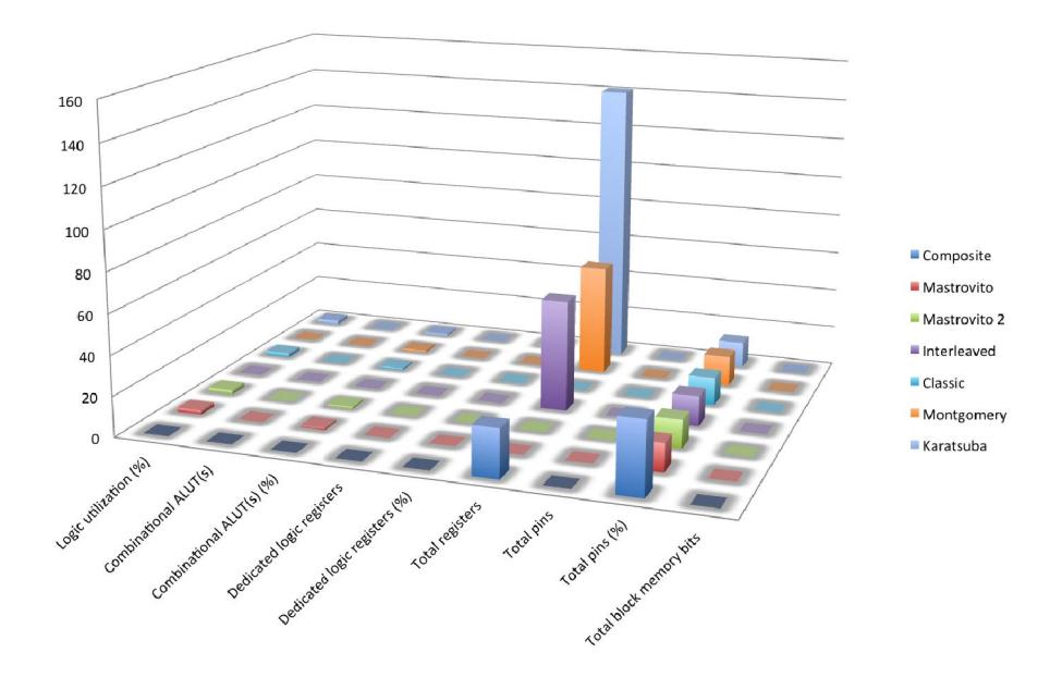
Figure 15 Multiplier Comparison.
| Composite | Mastrovito | Mastrovito 2 | Interleaved | Classic | Montgomery | Karatsuba | |
|---|---|---|---|---|---|---|---|
| Combinational ALUT(s) | 0.072916667 | 0.135416667 | 0.102564103 | 0.024839744 | 0.102564103 | 0.000224359 | 0.001498397 |
| Dedicated logic registers | 0.001923077 | 0 | 0 | 0.004407051 | 0 | 0.004407051 | 0.011298077 |
| ■ Total registers | 0.24 | 0 | 0 | 0.55 | 0 | 0.55 | 1.41 |
| Total pins | 0.355685131 | 0.139941691 | 0.139941691 | 0.151603499 | 0.139941691 | 0.151603499 | 0.128279883 |
Figure 16 Brief Multiplier Comparison.
6 Conclusions
Our multiplier has been compared with other multipliers and the result conforms our hypothesis that our multiplier gives better trade off for time and space, like shown in Figure 15 and Figure 16. The number of total pins is higher in order to lower the use of ALUT and registers.
The experiment results in Table 1 shows that composite field implementation requires less combinational ALUT and registers (area) than most of multipliers. This advantage achieved by gaining better trade off for time is space is the flexibility of the architecture design that can be modified to fit devices according to space of time available.
Acknowledgement
This research is supported by Hibah Kompetensi DIKTI based on SK Dekan STEI No. 0930/II.C07.1/DN/2011. We thank Muhammad Hafiz Khusyairi and Nopendri Zulkifli for their inputs and discussions on the topic.