
1 Introduction
A metropolitan area network (MAN) is a computer network that usually covers a city or a large campus, which has a geographic scope that falls between a wide area network (WAN) and a local area network (LAN). A MAN usually interconnects a number of nodes representing LANs that are interconnected using high-capacity backbone technology such as fiber optics, and provides uplink services to WANs and the Internet.
Some implementation technologies used for this purpose are the asynchronous transfer mode (ATM), the fiber distributed data interface (FDDI), and the switched multimegabit data service (SMDS). In most areas, these technologies are in the process of being displaced by ethernet-based connections (e.g., Metro Ethernet). MAN links between LANs have been built without cables using microwave, radio, or infrared laser links. Most companies rent or lease circuits from common carriers due to the fact that laying long stretches of cable can be expensive.
Distributed-queue dual-bus (DQDB) is the metropolitan area network standard for data communication that is specified in the IEEE 802.6 standard. Using
Copyright © 2012 Published by LPPM ITB, ISSN: 1978-3086, DOI: 10.5614/itbj.ict.2012.6.2.1
DQDB, networks can be up to 30 km long and operate at speeds up to 155 Mbit/s.
Point-to-point networking that supports MAN connections can be built based on network configurations such as a "bus" network, a "star" network, a "ring" network, or a "mesh" network. With the widespread dependence upon such networks, it becomes important to look for topologies that yield a high level of reliability and a low level of vulnerability to disruption. In this paper, the network configurations "wheel" and "fan" will be discussed.
It is desirable to consider quantitative counter-measures to address a network's vulnerability when designing a MAN. In order to obtain such measures we model the network by a graph in which the station terminals are represented by the nodes of the graph and the links by the edges. In what follows, we assume G = (V, E), a simple graph where V is the non-empty set of nodes, and E is the set of edges. We use the notation n(G) = |V| for the order of the graph G and e(G) = |E| for the size of the graph G. Unless specifically stated otherwise, we follow the standard graph theory notation found in [1].
Definition 1. The edge-connectivity of G, denoted by \(\lambda(G)\) or simply \(\lambda\), is defined to be \(\lambda(G) = \min\{|F|: F \in E, F \text{ is an edge failure set}\}\) [2].
One drawback of the traditional edge-failure model is that the graph G - F is an edge-failure state if it is disconnected and no consideration is given to whether or not there exists a "large" component that in itself may be viable.
It is reasonable to consider a model in which it is not necessary that the surviving edges form a connected sub-network as long as they form a sub-network with a component of some predetermined order. Therefore, we introduce a new edge-failure model, the k-component order edge-failure model. In this model, when a set of edges F fails we refer to F as a k-component edge-failure set and the surviving sub-network G - F as a k-component edge-failure state if G - F contains no component of order at least k, where k is a predetermined threshold value.
Definition 2. Let \(2 \le k \le n\) be a predetermined threshold value. The k-component order edge-connectivity or component order edge connectivity of G, denoted by \(\lambda_c^{(k)}(G)\) or simply \(\lambda_c^{(k)}\), is defined to be \(\lambda_c^{(k)}(G) = \min\{|F|: F \in E, F \text{ is } k \text{ - component edge failure set}\}\), i.e., all components of G - F have order \(\le k - 1\) [3],[4].
Definition 3. A set of edges F of graph G is \(\lambda_c^{(k)}\) -edge set if and only if it is a k-component order edge-failure set and \(|F| = \lambda_c^{(k)}\) [3]-[5].
From this short explanation, we offer the option of networks or graphs in designing a MAN network topology with vulnerability issues by computing \(\lambda_c^{(k)}(G)\) for a specific type of graphs.
2 Preliminary Results
get the following result [6].
The following networks suggest which MAN topology is the best option regarding its degree of vulnerability. The first type of graph we consider is the cycle, \(C_n\). The formula for \(\lambda_c^{(k)}(C_n)\) can be derived in a similar manner to that of \(\lambda_c^{(k)}(P_n)\) [3]. When one edge of the cycle is removed, it becomes a path with n nodes, \(P_n\). Thus \(\lambda_c^{(k)}(C_n) = \lambda_c^{(k)}(P_n) + 1\), and since \(\left\lfloor \frac{n-1}{k-1} \right\rfloor + 1 = \left\lceil \frac{n}{k-1} \right\rceil\) we
Theorem 1. Given \[2 \le k \le n\], \(\lambda_c^{(k)}(C_n) = \left\lceil \frac{n}{k-1} \right\rceil\) [4],[6].
The second type of network that has been considered is the complete graph on n nodes, \(K_n\). Let \(F \subseteq E(K_n)\) be a \(\lambda_c^{(k)}\) -edge set. We can compute |F| by calculating the maximum number of edges that can remain in the k-component edge-failure state \(K_n - F\). It is easy to see that any edge in F must have its endpoints in two different components of \(K_n - F\); therefore each component of \(K_n - F\) must itself be complete.
Lemma 2. Given \[2 \le k \le n\], let \(n = \left\lfloor \frac{n}{k-1} \right\rfloor (k-1) + r\) where \(0 \le r \le k-1\) [3]-[5].
From this it immediately follows that a maximum-size k-component edge-failure state of \(K_n\) consists of \(\left\lfloor \frac{n}{k-1} \right\rfloor\) complete components each of order k-1 and possibly one additional component of order less than k-1. Thus we have the following:
Theorem 3: Given \[2 \le k \le n\], \(\lambda_c^{(k)}(K_n) = \binom{n}{2} - \left\lfloor \frac{n}{k-1} \right\rfloor \binom{k-1}{2} - \binom{r}{2}\), where \(n = \left\lfloor \frac{n}{k-1} \right\rfloor (k-1) + r\), \(0 \le r \le k-2\) [1],[4],[5].
3 Main Results Model of Network Topology
The preliminary results suggest the network topologies wheel and fan. Since we do not have a formula or an algorithm that computes \(\lambda_c^{(k)}(G)\) of an arbitrary graph G representing the network, therefore we want to find bounds (both lower and upper) that may be applied to establish the range of possible values of \(\lambda_c^{(k)}(G)\). Before we introduce a set of bounds we need to establish some notation and terminology.
First we consider the value of \(\lambda_c^{(k)}(H)\), where H is a sub-network of G but H is not spanning or connected. If H is a graph on m nodes, and m < k, then every component of H has order \(\leq k-1\), so it follows that \(\lambda_c^{(k)}(H) = 0\). If H is disconnected and \(H_1, H_2, \cdots, H_p\) are the components of H, then
\[\lambda_c^{(k)}(H) = \sum_{i=1}^p \lambda_c^{(k)}(H_i).\]
Definition 4. If \(F \subseteq E\) is a set of edges, G[F] denotes the sub-network of G with node set V and edge set F, i.e. G[F] = G - (E - F) [4].
Definition 5. If U, \(W \subseteq V\) with \(U \cap W = 0\), [U, W] denotes the set of all edges with one endpoint in U and the other endpoint in W[4].
The next theorem is the basis of our lower bound.
Theorem 4. If \(E_1 \cup E_2\) is a partition of E, then \(\lambda_c^{(k)}(G[E_1]) + \lambda_c^{(k)}(G[E_2]) \le \lambda_c^{(k)}(G)\) [4].
Proof. Let \(D \subseteq E\) be a \(\lambda_c^{(k)}\)-edge set and let \(D_i = E_i \cap D, i = 1,2\). Since \(E_i - D_i \subseteq E - D\), each component of \(G[E_i] - D_i\) is contained in a component of G - D and therefore is of order \(\leq k - 1\). It follows that
\[\begin{split} &\lambda_c^{(k)}\big(G[E_i]\big) \leq \mid D_i\mid. \text{ Therefore } &\lambda_c^{(k)}\big(G[E_1]\big) + \lambda_c^{(k)}\big(G[E_2]\big) \leq \mid D_1\mid + \mid D_2\mid = \mid D\mid \\ &= \lambda_c^{(k)}(G)\,. \end{split}\]
Thus we obtain the following lower bound:
\[\lambda_c^{(k)} (G[E_1]) + \lambda_c^{(k)} (G[E_2]) \le \lambda_c^{(k)} (G)\], where \(E_1 \cup E_2\) is a partition of \(E\).
In particular if u is a node of full degree, then \((n-k+1)+\lambda_c^{(k)}(G-u)\leq \lambda_c^{(k)}(G)\).
Now let \(U \subseteq V\) be a set of nodes with |U| = k - 1. We construct a k-component edge-failure set as follows: delete all edges that connect U to the rest of the graph, and then delete edges from \(\langle V - U \rangle\) until all components have order \(\leq k - 1\). Thus we obtain the following upper bound:
\[\lambda_c^{(k)}(G) \le |[U, V - U]| + \lambda_c^{(k)}(\langle V - U \rangle)\], where \(U \subseteq V\) with \(|U| = k - 1\).
We will apply these bounds to compute \(\lambda_c^{(k)}(G)\), when G is either \(W_n\), the wheel of order n, or \(F_n\), the fan of order n.
Definition 6. The wheel of order n, \(W_n\), is the network or graph formed by connecting a single vertex to all the vertices of a \(C_{n-1}\) [4].
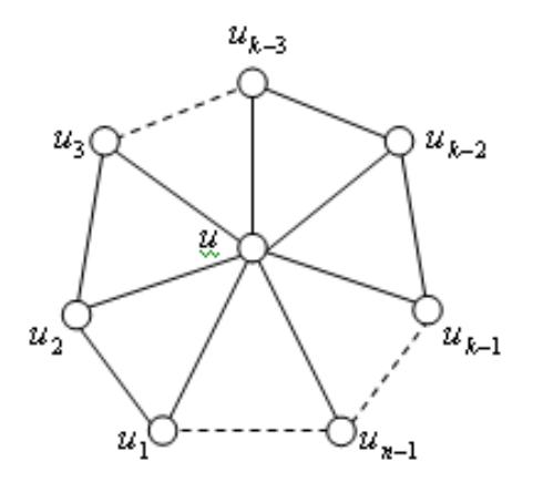
Figure 1 A wheel graph, \(W_n\).
Definition 7. The fan of order n, \(F_n\), is the graph formed by connecting a single vertex to all the vertices of a \(P_{n-1}\) [4].
Figure 2 A fan graph, \(F_n\).
Since the application of the bounds to \(W_n\) and \(F_n\) are done similarly, we will only demonstrate them for \(W_n\) and state the corresponding result for \(F_n\).
Let \(G = W_n\) and let u be the full degree node. Then \(G - u = C_{n-1}\) and the lower bound implies
\[\lambda_c^{(k)}(W_n) = \lambda_c^{(k)}(G) \ge (n - k + 1) + \lambda_c^{(k)}(C_{n-1}) = (n - k + 1) + \left\lceil \frac{n - 1}{k - 1} \right\rceil. \tag{1}\]
Now if \(U = \{u, u_1, \dots, u_{k-2}\}\) \(V - U = \{u_{k-1}, \dots, u_{n-1}\}\), then [U, V - U] = (n-1) - (k-2) + 2 = n - k + 3 and \(\langle V - U \rangle = P_{n-k+1}\). Thus the upper bound implies
\[\lambda_c^{(k)}(W_n) \le (n-k+3) + \lambda_c^{(k)}(P_{n-k+1}) \le (n-k+3) + \left| \frac{n-k}{k-1} \right|. \tag{2}\]
Inequalities (1) and (2) together yield the following bounds on \(\lambda_c^{(k)}(W_n)\):
\[(n-k+1) + \left\lceil \frac{n-1}{k-1} \right\rceil \le \lambda_c^{(k)}(W_n) \le (n-k+3) + \left\lfloor \frac{n-k}{k-1} \right\rfloor. \tag{3}\]
We will find the formula for \(\lambda_c^{(k)}(W_n)\) by comparing the lower and upper bounds.
\[(n-k+1) + \left\lceil \frac{n-1}{k-1} \right\rceil \le (n-k+3) + \left\lfloor \frac{n-k}{k-1} \right\rfloor\]. Subtracting \((n-k+1)\) from each side gives
\[\left\lceil \frac{n-1}{k-1} \right\rceil \le 2 + \left\lfloor \frac{n-k}{k-1} \right\rfloor. \tag{4}\]
Applying the division algorithm we write \(n-k=\alpha(k-1)+r\), where \(0 \le r \le k-2\), thus \(\alpha = \left\lfloor \frac{n-k}{k-1} \right\rfloor\). Hence n-1=(n-k)+(k-1) \(= \alpha(k-1)+(k-1)+r=(\alpha+1)(k-1)+r\). If \(r \ge 1\), i.e., (k-1) does not divide (n-1), then \(\left\lceil \frac{n-1}{k-1} \right\rceil = \alpha+2 = \left\lfloor \frac{n-k}{k-1} \right\rfloor + 2\). If r=0, i.e., (k-1) divides (n-1), then \(\left\lceil \frac{n-1}{k-1} \right\rceil = \alpha+1 = \left\lfloor \frac{n-k}{k-1} \right\rfloor + 1\).
Theorem 5. Let \(G = W_n\) be a wheel on n-nodes then [4],
\[\lambda_c^{(k)}(W_n) = \begin{cases} (n-k+1) + \left\lceil \frac{n-1}{k-1} \right\rceil, & \text{if } (k-1) \text{ does not divide } (n-1) \\ (n-k+2) + \left\lceil \frac{n-1}{k-1} \right\rceil, & \text{if } (k-1) \text{ divides } (n-1). \end{cases}\] (5a)
Proof. By using bound (3),
\[(n-k+1) + \left\lceil \frac{n-1}{k-1} \right\rceil \le \lambda_c^{(k)}(W_n) \le (n-k+3) + \left\lfloor \frac{n-k}{k-1} \right\rfloor\]
If (k-1) does not divide (n-1) then
\[(n-k+1) + \left\lceil \frac{n-1}{k-1} \right\rceil = (n-k+1) + \left\lfloor \frac{n-k}{k-1} \right\rfloor + 2 = (n-k+3) + \left\lfloor \frac{n-k}{k-1} \right\rfloor\]
Thus, if (k-1) does not divide (n-1), \(\lambda_c^{(k)}(W_n) = (n-k+1) + \left\lceil \frac{n-1}{k-1} \right\rceil\) and (1) holds.
If (k-1) divides (n-1) then
\[(n-k+1) + \left\lceil \frac{n-1}{k-1} \right\rceil = (n-k+1) + \left\lceil \frac{n-k}{k-1} \right\rceil + 1 = (n-k+2) + \left\lceil \frac{n-k}{k-1} \right\rceil\]
thus
\[(n-k+1) + \left\lceil \frac{n-1}{k-1} \right\rceil \le \lambda_c^{(k)}(W_n) \le (n-k+2) + \left\lfloor \frac{n-k}{k-1} \right\rfloor.\]
Claim. If (k-1) divides (n-1) then if we remove at most \((n-k+1) + \left\lceil \frac{n-1}{k-1} \right\rceil\) edges from \(W_n\) we do not get a k-component edge-failure state. Let
\(\left\lceil \frac{n-1}{k-1} \right\rceil = \beta\), if we remove \(\beta\) edges from the \(C_{n-1}\) we get \(\beta\) components and in order to have a k-component edge-failure state each has at most k-1 nodes. Since (k-1) divides (n-1) each must have exactly k-1 nodes. Thus we need to isolate the full degree node u from the \(C_{n-1}\), which means we must delete (n-1) additional edges. Hence we must remove at least \(\beta+1\) edges from the \(C_{n-1}\). Since \(\beta+1=\left\lceil\frac{n-1}{k-1}\right\rceil+1\) can remove at most (n-k) edges from the full
degree node which leaves at least k-1 edges remaining from u to the \(C_{n-1}\) and thus there is a component of order at least k.
Thus if \[(k-1)\] divides \((n-1)\) then \(\lambda_c^{(k)}(W_n) = (n-k+2) + \left\lceil \frac{n-1}{k-1} \right\rceil\) and (2) holds.
As previously stated the formula for \(\lambda_c^{(k)}(F_n)\) can be derived in a similar manner as that for \(\lambda_c^{(k)}(W_n)\), so the following result is stated without proof.
Theorem 6. Given \(2 \le k \le n\), then [4],
\[\lambda_c^{(k)}(F_n) = \begin{cases} (n-k+1) + \left\lfloor \frac{n-2}{k-1} \right\rfloor, & \text{if } (k-1) \text{ does not divide } (n-1) \\ (n-k+2) + \left\lfloor \frac{n-2}{k-1} \right\rfloor, & \text{if } (k-1) \text{ divides } (n-1) \end{cases}\]
4 Conclusion
The primary results discussed in [3] suggest investigation of new network models that make it possible to design aMAN network topology with the best solution for vulnerability issues.
When comparing network configurations with the same number of stations or nodes that need to be installed, a complete network is the best topology, but this makes it impossible to design a real MAN network. The cycle network is the simplest one in terms of installation, but it yields the worst results in terms of network vulnerability. We can see the comparison results in Table 1 below, which is based on the assumption that a MAN network is established with 10 stations or nodes, while k = 4, 5 and 6, respectively.
Table 1 Results of vulnerability comparison between different network configurations (cycle, complete, wheel and fan) with the same number of nodes.
| Туре | Formula | k = 4 | k = 5 | k = 6 |
|---|---|---|---|---|
| \(\lambda_c^{(k)}(C_{10})\) | \[\lambda_c^{(k)}(C_n) = \left\lceil \frac{n}{k-1} \right\rceil\] | 4 | 3 | 2 |
| \(\lambda_c^{(k)}(K_{10})\) | \[\lambda_c^{(k)}(K_n) = \binom{n}{2} - \left\lfloor \frac{n}{k-1} \right\rfloor \binom{k-1}{2} - \binom{r}{2}\] | 36 | 34 | 25 |
| \(\lambda_c^{(k)}(W_{10})\) | \[\lambda_c^{(k)}(W_n) = \begin{cases} (n-k+1) + \left\lceil \frac{n-1}{k-1} \right\rceil, & \text{if } (k-1) \text{ does not divide } (n-1) \\ (n-k+2) + \left\lceil \frac{n-1}{k-1} \right\rceil, & \text{if } (k-1) \text{ divides } (n-1) \end{cases}\] | 11 | 9 | 7 |
| \(\lambda_c^{(k)}(F_{10})\) | \[\lambda_c^{(k)}(F_n) = \begin{cases} (n-k+1) + \left\lfloor \frac{n-2}{k-1} \right\rfloor, & \text{if } (k-1) \text{ does not divide } (n-1) \\ (n-k+2) + \left\lfloor \frac{n-2}{k-1} \right\rfloor, & \text{if } (k-1) \text{ divides } (n-1) \end{cases}\] | 10 | 8 | 7 |