
1 Introduction
In many applications, there is often a need to track rectangular and quadrangular objects. For example, in our previous work, there is a need for detecting and tracking quadrangles from images to assist the projector-camera system for displaying virtual objects on a piece of white card board or paper [1]-[2].
In such a system, a camera and a projector are mounted together and facing the same direction.as in Figure 1. A user can move the board freely at a distance away and the camera is capturing and calculating the position of the board relative to the camera-projector pair. Hence, the desired image can be projected correctly onto the board. The user can freely move this very lightweight board as an interface to the computer to view movies, pictures etc. There are plenty of applications for such systems. For example, it can be used for a passenger in a flight to watch movies, so the user does not need to view the fixed TV panel in front of him. Moreover, this can also be used as a teaching tool for medical students, in that the student doctor can examine the internal view of a human
body by moving the board up and down to select the correct cross-sectional view of the target object. The application potential for this setup is enormous. To achieve the above goal, we need to detect the board, which appears to be a quadrangle in the image captured by the camera. Therefore, a robust quadrangle detector is required. However, the previous system has a time lag problem, when the board is moving too fast the detection may take up to 0.5 seconds to complete, hence the image may appear to be lagging behind the board. Therefore, a more efficient algorithm for quadrangle detection is a necessity. In previous systems, the Canny edge detector and Hough line transform [1]-[3] are used to obtain the line features. Then an exhausted search over the line combinations is carried out to find four lines which can form a good quadrangle. Finally, the four corners of the detected quadrangle are tracked with a particle filter. Other approaches such as the one by Zhang's [4] is slightly different; it projects the edge map from a Sobel edge detector to the Hough space and carries out the exhausted search directly in the Hough space. Then, when a quadrangle is detected, dynamic programming is employed to track the pose and location of the detected quadrangle. We think that although these detection methods can achieve acceptable results, the performance can certainly be improved by adding Kalman filter based tracking.
Figure 1 The camera projector system used in our previous work [1]-[2].
We found that line tracking by Kalman filter (KF) [5] and extended Kalman filter (EKF) have been investigated in the work of Mills [6]-[7], the tracking procedure is performed in the Hough space for reliable line tracking even partial occlusion exists. And in [8], Condensation [9] is also employed for tracking the set of lines in the Hough space. However, poor modeling in the Kalman filter may lead to large estimation error [10]. For example, if the line is too close to the origin, Hough-based feature detection (that Kalman filter depends on) would be difficult to function. To address this problem, a mathematical scheme called Multiple Model Adaptive Estimation algorithm (MMAE) is proposed to be used [11] and the Multiple Model Kalman filter (MMKF) is used as a stochastic version of MMAE in [11] and [12]. In this paper, we investigate the use of MMKF and apply it to line tracking. We believe the MMKF is useful to improve the robustness and stability with little sacrifice of speed. The proposed MMKF method is not only useful for tracking lines but may also be extended to handle other shapes such as polygons etc. We believe using this method we can produce a robust line detector for even for low-cost mobile camera-projector systems. Hence, a quadrangle detector based on this line detector can be achieved. In Section 2, the rationale and the design of our method will be discussed. Section 3 is about the details of the implementation. Experimental results are discussed in Section 4 and we conclude the whole paper in Section 5.
2 Theory and Design
2.1 Introduction to Quadrangle Detection and Tracking
In many applications such as a projector-camera system [1], the display content has to be projected onto the correct display rectangular area. To achieve this, the system must able to locate the display area and find out the pose of it. Since the display area can move freely in the 3D camera view frustum and the projection frustum, the rectangular display area is likely to be deformed into a quadrangle by a perspective transformation. Therefore, we need a method to search for quadrangles, which are built from lines. Hence, a robust line detector is needed in such applications.
2.2 Definition of a Quadrangle
As mention in the previous section, the display area we targeted is a rectangle. However, this rectangle is deformed into a quadrangle by perspective transformation. The i-th quadrangle Qt,i is considered as a set of 4 straight lines extracted in the image It at time t and described as { , ,, } ,it p tsrq Q = l l l l ,where lp, lq, lr , ls , are the distinct lines in the image It at time t and they are arranged in an anti-clockwise order. A quadrangle is shown in Figure 2(b).
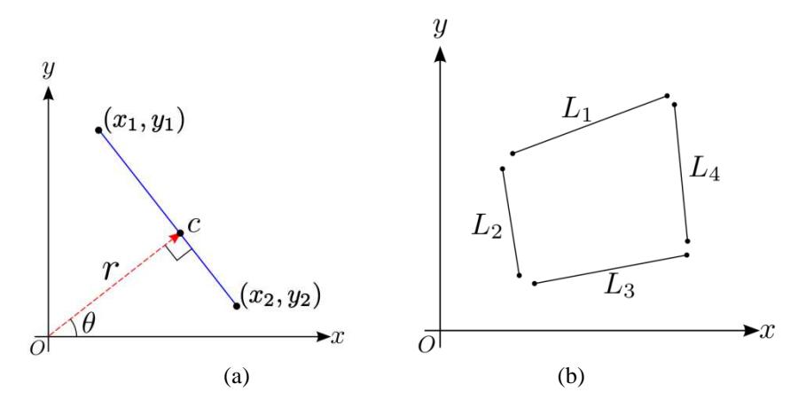
Figure 2 (a) Graphical illustration of the definition of a line. (b) Illustration of the quadrangle defined from lines Lp, where p=1, q=2, r=3, s=4.
2.3 Line Feature Extraction in our system
The line feature is extracted by first using Progressive Probabilistic Hough transform (PPHT) [13]. It takes a binary edge image as input and output a set of lines that has votes larger than a threshold. There are two more parameters, the minimum line length and the maximum gap length. The minimum line length not only specifies the type of line the algorithm output but also suppresses false positive output. Due to rounding error, a long line segment may be decomposed into many short line segments. The maximum gap length helps joining those short line segments together. The threshold, the minimum line length and the maximum gap length are specified by the user. However, the values of the parameters are dependent on the application and the scene. Hence, the user has to adjust the values for different applications and scenes. Unlike the original Hough Transform, PPHT has a shorter execution time and, therefore, it is used in our application. On the other hand, PPHT returns the two end points of the lines while the original Hough Transform returns the lines in the form of \(r,\theta\)pair. Although extra steps have to be taken to find the \(r,\theta\) value in PPHT, it is still faster than finding the two end points using the edge map and \(r, \theta\) pair.
2.4 Automatic Quadrangle Detection
If the system is designed for graphic display applications such as that in [1], the quality of the image projected on the surface is important. To facilitate a good projection, the rotation angle of display area should not be too large. Moreover, the distance between the projector-camera pair and the display should be in a proper range. It is because if the projector is too far away, the projected image might not be bright enough for human eyes under bright environment. If they are too close, the whole display area might not be seen by the camera. Therefore, we put a upper limit and a lower limit on the length of \(l_p\), \(l_q\), \(l_r\) and \(l_s\). The corners of the quadrangle should also be inside the camera view. Because this quadrangle is a deformed rectangle by perspective transformation and the rotation of the display area is small, we observed that there are some useful properties in the quadrangle for detection. With the help of those properties, the system can quickly locate the quadrangle (instead of exhaustively exploring every quadrangle) found in the image.
Therefore, our aim is to develop a set of rules for quadrangle detection. The first observed property is that the opposite sides are almost parallel. The angle between the lines \(l_p\), \(l_r\) of the quadrangle is small. Moreover, it is true for the line \(l_q\) and \(l_s\). Similarly, the second property is that the adjacent sides are almost perpendicular to the each other. That means the angle between the adjacent lines is around \(90^\circ\). The last property is the ratio between the adjacent sides. These ratios are close to the original rectangle. We derived the detection criteria from all these observations. A candidate of the possible display area is a quadrangle that passes the detection criteria as follows:
- 1. The opposite sides are almost parallel.
- 2. The adjacent sides are almost perpendicular to each other.
- 3. The corners of the quadrangle should be inside the image.
- 4. The lengths of the four sides are within the lower limit to the upper limit.
- 5. The ratio between the adjacent sides is close to the display area.
In Figure 3, (a) is the image frame captured, (b) is the edge map produced by using Canny edge detector, (c) is the lines detected using progressive probabilistic Hough transform and (d) is the result of drawing the lines on current frame. Lines are extracted from the image. Let us assume N lines were found in the current image frame \(I_t\). The total number of quadrangles can be formed by all these N lines is
\[\binom{N}{4} = \frac{N!}{4!(N-4)!} = \frac{N(N-1)(N-2)(N-3)}{4!}\] (1)
Since the number of quadrangles grows with \(O(N^4)\), it is impractical to examine all the quadrangles. Instead of using all N lines to form quadrangles, the system can select distinctive lines, uses them to construct quadrangles and tests them with the criteria. We observed that a long strong edge may be divided into multiple short lines during the line detection phase. These small segments will induce a lot of duplicated parallel line pairs and perpendicular line pairs. All the duplicated line pairs are referring to the same line pair formed with the same strong edges. Therefore, the time spend on the calculation on the duplicated line
pairs is wasted. To overcome this problem, data clustering techniques will first be applied to the set of lines and similar lines are put into the same cluster. Similar lines are determined by calculating the similarity score defined as the following.
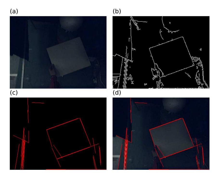
Figure 3 Edge points and lines extracted from a real image.
The similarity measurement \(S(l_i, l_j)\) is the Euclidean distance between the closest point of the two line \(l_i\) and \(l_i\). The closest point \(c_i\) of the line \(l_i\) is
\[(r_i \cos(\theta_i), r_i \sin(\theta_i)), hence\]
\(S(l_i, l_j) = S(l_j, l_i) = \sqrt{(c_i - c_j)(c_i - c_j))}\)
The lines are similar if and only if \(S(l_i, l_i) \le threshold\)
Similarly, we can define lines that are (i) parallel, (ii) perpendicular in a similar fashion. Therefore those lines that satisfy parallel and particular criteria will be grouped together to become quadrangles.
2.5 Line Tracker and the Problem when the Line is Close to the Origin
A line segment can be defined by its two end-points. However, occlusion of these two end-points is unavoidable in many real world situations. In this paper, a line L is represented by using the conventional polar coordinates of r and \(\theta\) [3]. The point C is the closest point between the line and the origin (of the coordinate system used), and r is the shortest distance between the origin to C. In addition, \(\theta\) is the angle between the horizontal axis and the vector from the origin to C. The x-y coordinate of C is tracked using the Kalman filter.
A single Kalman filter scheme alone cannot yield good result especially when the target line is near (e.g. r is only a few pixel long) or almost passing through the origin. To solve this problem, we propose to use multiple independent Kalman filters to track a line, i.e., each Kalman filter uses a different coordinate system with a different center (origin). To make this effective, we need to select the relative positions of the N (\(\geq 3\)) coordinate systems so that the origins are not collinear. The effect is even if a line is close to the origin(s) of one or two coordinate systems it would be far away from the origins of the other coordinate systems. We believe that by using this multiple models scheme, the prediction accuracy and reliability can be improved.
2.6 Kalman Filter Design
The x,y coordinates of the closest point C of a line L is being tracked using the Kalman filter (KF). We assume the closest point is moving with a constant acceleration, and the motion in both x-axis and y-axis are independent and linear. The motion of the closest point C can be described using the equation of motion as follows:
\[x_{t} = x_{t-1} + \dot{x}_{t-1} \Delta t + \frac{1}{2} \ddot{x}_{t-1} \left( \Delta t \right)^{2}\] \[\dot{x}_{t} = \dot{x}_{t-1} + \ddot{x}_{t-1} \Delta t\] \[y_{t} = y_{t-1} + \dot{y}_{t-1} \Delta t + \frac{1}{2} \ddot{y}_{t-1} \left( \Delta t \right)^{2},\] \[y_{t} = \dot{y}_{t-1} + \ddot{y}_{t-1} \Delta t\] (2)
where \(x_t\), \(\dot{x}_t\) and \(\ddot{x}_t\) are the displacement, velocity and acceleration respectively of the closet point C in frame i in the x-direction. Similarity, \(y_t\), \(\dot{y}_t\) and \(\ddot{y}_t\) are the displacement, velocity and acceleration respectively of the closet point C in frame i in the y-direction. \(\Delta t\) is the time interval between two consecutive
frames. The state matrix and the measurement matrix of the Kalman filter at time t are:
\[X_{t} = \begin{bmatrix} x_{t} & \dot{x}_{t} & y_{t} & \dot{y}_{t} \end{bmatrix}^{T}, \ Z_{t} = \begin{bmatrix} x_{t} & y_{t} \end{bmatrix}^{T}\] \[(3)\]
Derived from the equations of motion, the state transition model A and the observation model H are:
\[A = \begin{bmatrix} 1 & \Delta t & 0 & 0 \\ 0 & 1 & 0 & 0 \\ 0 & 0 & 1 & \Delta t \\ 0 & 0 & 0 & 1 \end{bmatrix}, \quad H = \begin{bmatrix} 1 & 0 & 0 & 0 \\ 0 & 0 & 1 & 0 \end{bmatrix}\](4)
\[Q = \begin{bmatrix} \frac{(\Delta t)^4}{4} & \frac{(\Delta t)^3}{2} & 0 & 0\\ \frac{(\Delta t)^3}{2} & (\Delta t)^2 & 0 & 0\\ 0 & 0 & \frac{(\Delta t)^4}{4} & \frac{(\Delta t)^3}{2}\\ 0 & 0 & \frac{(\Delta t)^3}{2} & (\Delta t)^2 \end{bmatrix}, R = \begin{bmatrix} 0.5 & 0\\ 0 & 0.5 \end{bmatrix}\] (5)
Where the noise covariance is Q and measurement noise covariance is R.
2.7 Our Multiple-Model Kalman filter Line Tracing Algorithm
The multiple-model Kalman filter (MMKF) paradigm is used in our tracker. Figure 4 shows the overview of our line tracker. \(Z_k\) is the measurement at time k. And it is transformed to the coordinate system of the i-th Kalman filter (denoted as \(KF_i\)) by the transformation \(T_i\) into \(Z_{k,i}\). State \(X_{k,i}\) is the prediction of the state of the closest point in the next frame by the i-th Kalman filter. All the prediction results are transformed back to one common coordinate system by applying the corresponding inverse transformation \((T_i)^{-1}\). Finally, a line fitting function will be applied to find the final prediction of the line.
The advantage is discussed in [12]. In our tracker, each filter uses a different coordinate system. And if the origins of all these coordinate systems are not collinear (as discussed earlier), the line cannot pass through these origins at the same time. This is to ensure that even when r in one model is small, the values of r in other models are large enough to give a correct result. The prediction of each sub-Kalman filter is the position and velocity of the closest point. By discarding the velocity terms, we can obtain a set of closest (C) points that should lie on a straight line as shown in Figure 3(a). We can use a least squares fitting method to find a best fit line that minimizes the sum of square errors among the line and closest (C) points.
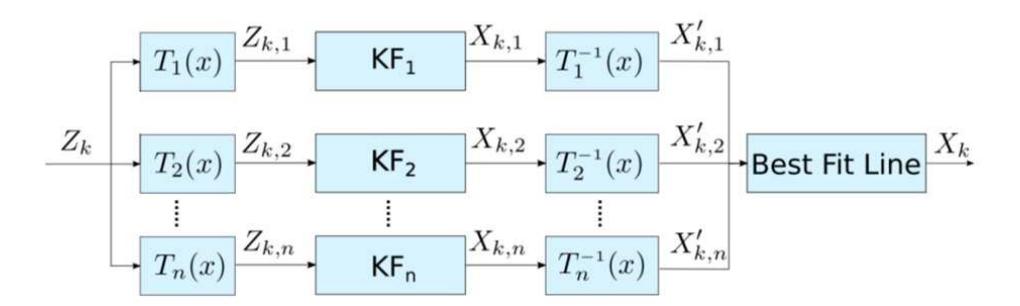
Figure 4 The overview of the line tracker. KFi=the i-th Kalman filter.
3 Experiments
To evaluate the robustness and stability of our proposed trackers, we generate a set of synthetic data to simulate different kinds of movements, e.g. motion with small r and complex motions with mixed translation or rotation. In the data set, the two end-points of the lines are given. The length of the line is not fixed for some data set to simulate the lines extracted in real images. The overlap ratio, defined in [12], is used to evaluate how good the line tracker is performing. We first draw the predicted line (ground truth) with n pixels thick (it becomes a ground truth range of a line) and draw the line found by our algorithm on top of it.
The overlap ratio is the percentage of the number of pixels of the line detected inside the ground truth range over the total number of pixels of the line detected. If the line found is completely inside the ground truth range, the overlap ratio is 100% and so on. The width of the ground truth range is to provide a certain tolerance for the results. Because there may be error accumulated in different processes like Canny edge detection, Hough transform and rounding error in the calculation. The width is set to 2 pixels throughout all the experiments conducted, see [12] for details of the definition of overlapping ratio.

Figure 5 Overlap ratio in Pure translation. Our approach is 3KF.
3.1 Experiment 1: Translation performance
To compare the performance between trackers, 20 randomly generated line segments with pure translation motion in 24 directions (0°, 15°, 30° and so on until 345°) and 3 different speeds (1, 2, 3 pixels per frame) are tested. The trackers are tested in 20 consecutive frames. The average score of all lines in the same directions are shown in Figure 5. We can see that the proposed 3KF can slightly improve the performance in term of accuracy and stability.
3.2 Experiment 2: Rotation performance
In this experiment, the value of r of the line is fixed to 10, 50 and 100 pixels. For each value of r, the angular velocity is set to \(1^{\circ}\), \(2^{\circ}\), \(4^{\circ}\), \(8^{\circ}\) and \(16^{\circ}\) degrees per frame. We record the performance of the trackers in 20 frames. The average scores are shown in Figure 6. The score of 3KF drops below 20% when the angular velocity reaches 4 degrees per frame and higher for all tested value or r.
3.3 Experiment 3: Real video test
In a real video test, a white cardboard is put on a silver screen so that the cardboard can be easily detected. The camera is moving freely but slowly. Figure 7, in the first row, the left picture shows the snapshot of the system at frame 41 of the testing video, the right picture shows the quadrangle detected. Figure 8 shows the case for frame 42. The system is now using the predictions of the trackers to form the quadrangle.
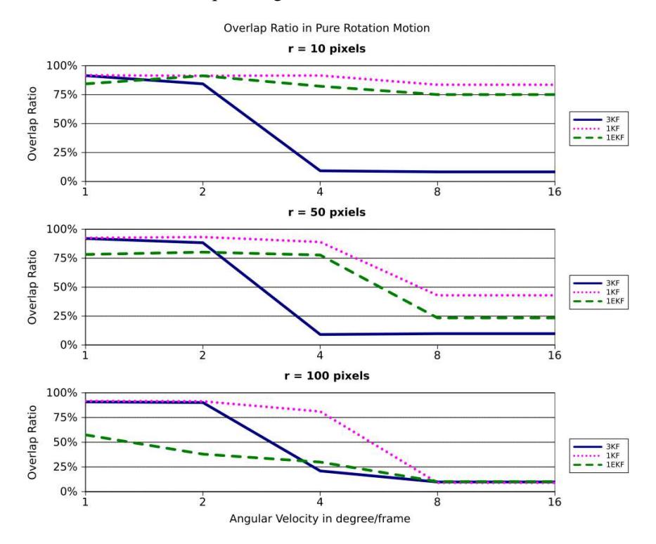
Figure 6 Overlap ratio in pure rotation motion. Our approach is 3KF.
Figure 7 Lines (left) and a quadrangle (right) is detected and shown at frame 41.
Figure 8 shows the case for frame 43 of the sequence. The system failed to extract lines for the top and bottom of the board. However, we can use the prediction ability of the trackers for the top side and bottom side to form a quadrangle using our Real-time Quadrangle Tracking Method mentioned in section 2.
Figure 8 Lines detected and a quadrangle le is tracked at frame 43.
4 Conclusion
The work investigates how we can robustly detect and track a quadrangle in real time. Since a quadrangle composed of four lines, so a robust line tracker is required. A line tracking method adopting the Multiple Model Kalman filter paradigm is proposed in this paper. Each Kalman filter works on a state transition scheme based on a particular coordinate system. By combining all the outputs of these Kalman filter modules, we can produce robust line tracking results. In our tests, we show that our three-Kalman method outperforms the use of a single-Kalman or two-Kalman filter schemes especially when the line is close to the origins of one or two coordinate systems. It is also suggested that the choices of the locations of the coordinate systems may affect the performance, and selection of these coordinates may be a future research direction. The lines detected are then used for quadrangle detection. Our algorithm is also very efficient, and even a small embedded system can process a line at 200 frames per second. We believe using this method can produce a robust line and quadrangle detection module for low-cost mobile applications. The next step is to merge it with our existing camera-project based handheld display system [1] to improve its speed and accuracy. As mentioned in the introduction there is time-lag problem when the board is moving too fast, we hope this efficient quadrangle can solve this problem. Moreover, we are also exploring a hardware approach for line detection and quadrangle detection.. As we have seen, the line detector requires the Canny edge detector which takes up a heavy resource for the calculation of the image gradients. We found that image gradients can be easily calculated by simple subtraction of pixel values
direction sent from the camera image bit stream, and it can be implemented by logic gates using an FPGA (field programmed gate array) by a hardware language VHDL or VERILOG. The advantage is not only it is efficient, it is also economical and power saving because expensive and power-hungry math processors can be replaced by simple logic gates. So, our projector-camera system can be easily integrated into mobile phones or other mobile devices.
Acknowledgement
This work is supported by a direct grant (Project Code: 2050455) from the Faculty of Engineering of the Chinese University of Hong Kong.