
1 Introduction
In the design of satellite communications systems there are several aspects that should be considered. The two most important are frequency allocation and ground station location, which influence signal penetration and propagation. If the allocated frequency is too low, the signal will have difficulty penetrating the ionosphere. On the other hand, if it is too high the signal will suffer more attenuation due to its natural behavior in relation to the wavelength, which causes a decrease in amplitude, radio-wave depolarization, and an increase in thermal noise [1]. Nevertheless, the use of high-frequency allocation is unavoidable for broadband satellite communication since high data rates, such as used by enhanced video and data services, need to be supported by a large bandwidth. Therefore, the use of a frequency allocation higher than C-band and Ku-band, such as K-band, is required to fulfill the bandwidth requirement as well as to overcome the congestion problems that often occur in the conventional C-band or Ku-band. Unfortunately, as the allocated frequency is above 10 GHz it is susceptible of being affected by atmospheric conditions, especially rain conditions [1]-[2]. This is a serious issue for some countries located in tropical areas such as Indonesia, since two-thirds of the world's rain falls in this area and affects higher rain rates compared to non-tropical areas.
There is still little research related to rain propagation attenuation concerned with developing rain models for terrestrial communication [3]-[5]. Some attempts have been made at the simulation of an overview of rain attenuation, fade slope, and fade duration with three models [3]. The simulation used measured rain rate data covering three months from Surabaya (city), Indonesia. In [4], two algorithms for estimating the distribution of rain events and link fades used data gathered in the South East of the United Kingdom over three years. The first algorithm converted the distribution of rain durations into the distribution of link fade duration. The second one exploited features of the spatial and temporal power spectrum of the rain rate predicted by models of turbulence. Moreover, the development of channel modeling in a time series is investigated [5]. This investigation considers the impact of rain rate on microwave attenuation, fading and wave polarization propagation millimeter for the 30 GHz frequency and assumes that the channel is a random variable.
Furthermore, channel-modeling research regarding a propagation model of satellite channels in non-tropical areas has been undertaken in [6]-[8]. A new stochastic-dynamic model for planning and designing gigahertz satellite communications has been investigated using fade mitigation techniques in [6]. It was assumed that the stochastic-dynamic model is a generalization of the Maseng-Bakken model so that the outcome is a model that is capable of yielding theoretical descriptions of the long-term power spectral density of rain attenuation, rain fade slope, the rain frequency scaling factor, site diversity, and fade duration statistics using a novel method based on Markov chains. A method for predicting the fading properties of satellite-to-earth propagation channels using Markov models has been proposed in [7]. The same method is also applicable to evaluate the performance of error probability by use of coherent QPSK modulation schemes for satellite mobile communication services. In [8], the design and implementation of automated rain-fade simulation and power augmentation systems on a 20 GHz communications link
using a multimode traveling wave tube amplifier for loss compensation are presented.
The organization of this paper is as follows. In Section 2, the development of a method for predicting rain attenuation and rain propagation attenuation for high frequencies in K-band satellite communications link application is described. Here, the method applied to predict rain rate and attenuation is based on the hidden Markov model (HMM). Section 3 analyzes the prediction results of the proposed method, which are then compared with the measured data and the models in recommendation ITU-R P.837-5 [9] and recommendation ITU-R P.618-10 [10] for rain rate and rain propagation attenuation respectively. The statistical distribution for fade and interfade duration compared with recommendation ITU-R P.1623-1 [11] is also discussed in Section 3. Finally, Section 4 concludes the paper.
2 Rain Attenuation and Rain Propagation Attenuation
In the electromagnetic spectrum, the K-band frequency ranges from 18 GHz to 26.5 GHz. The advantages of using K-band rather than lower frequency bands are the availability of a larger bandwidth to obtain a higher system capacity and a smaller antenna size to achieve the same gain. However, a disadvantage is that it requires more power for transmitting the signal to cope with attenuation regarding atmospheric conditions. This is because K-band signals are often attenuated by rain droplets, gas, clouds and ice particles and because the noise temperature in the receiver increases. The dimension of the wavelength for frequency bands above 10 GHz is similar to that of a rain droplet, which implies that the signal at these frequency bands is very easily absorbed by the rain. Rain attenuation has become one of the most important factors that can prevent the signal level at the receiver from achieving the sensitivity level. Meanwhile, other factors that contribute to the increase of the attenuation are elevation angle, altitude angle, and antenna polarization.
2.1 Rain Attenuation
In K-band satellite communications links, rain affects signal propagation in three ways: it attenuates the signal, increases the system noise temperature, and changes the signal polarization [12]. All of these aspects decrease the received signal quality. At lower frequencies, such as C-band, these effects are insignificant. However, they become increasingly significant as the frequency increases. At the Ku-band, the effect can still be accommodated with some effort. However, K-band and higher frequencies initiate a huge degradation, which simply cannot be compensated at the level of availability that is usually expected at lower frequencies.
Rain attenuation is caused by the scattering and absorption of electromagnetic waves by rain droplets. The scattering diffuses the signal, while absorption involves resonance of waves with individual molecules of water. Absorption increases the molecular energy, corresponds to a slight increase in temperature, and results in an equivalent loss of signal energy. Attenuation is negligible for snow or ice crystals, in which the molecules are tightly bound and do not interact with the waves. In terms of rain, the attenuation increases as the wavelength approaches the size of a raindrop, typically about 1.5 mm. For Cband (wavelength = 37.5 mm to 75 mm) and Ku-band (wavelength = 16.67 mm to 25 mm), the wavelength is 10 to 50 times larger than a raindrop and the signal passes through the rain with relatively insignificant attenuation. However, in K-band (wavelength = 11.42 mm to 16.67 mm), the wavelength approaches the rain droplet size significantly, which affects a quite large amount of attenuation.
The standard formula for rain attenuation (Lr) in dB fulfills (1) [1],
\[L_r = \alpha R^{\beta} L = \gamma L \tag{1}\] where R, L and γ are: rain rate (mm/h), equivalent path length (km), and specific rain attenuation (dB/km) respectively, while α and β are empirical coefficients that depend on frequency. In correlation with satellite communications links, the value of the equivalent path length depends on the elevation angle of earth station to satellite, rain height and latitude of earth station. When the rain rate increases, i.e. rather heavy rain, the rain droplets become larger, so there is more attenuation. Two authoritative, widely used rain models are the ITU-R (CCIR) model and the Crane model [1].
2.2 Rain Propagation Attenuation
In this paper, the method applied to predict the rain rate and rain attenuation propagation is the hidden Markov model (HMM). To simplify the model, it was assumed that rain with some intensity has a certain probability value of occurrence. Similarly, the rain propagation attenuation also has a certain probability, which depends on rain intensity. Values of probability were obtained from measurements in the field with specific parameters. The hidden Markov model can be described as {S, A, Ψ, P, F}, where S is channel state space, A is output that can be observed, Ψ is initial state matrix, P is transition probability matrix, and F is probability of observing a symbol or emission matrix.
The transition from state i to state j that produces an output symbol a can be formulated as in (2).
\[\mathbf{P}\{a_i\} = P\{a, j|i\} \tag{2}\]
Hence, the probability to produce sequence a, is expressed in (3).
\[P\{a_1^t\} = \Psi \prod_{i=1}^t \mathbf{P}\{a_i\} \mathbf{1}\] (3)
where the elements of \(P\{a_i\}\) are defined as written in (4).
\[\mathbf{P}\{a_i\} = P\{a, j|i\} = P\{j|i\}P\{a|i, j\}\] \[\tag{4}\]
Similar to the previous investigation [13], a model to predict rain rate and propagation attenuation is proposed based on HMM using time series measurement data. In principle, the model groups the rain rate and rain propagation attenuation into a number of classes. By using HMM, the group of rain rate and the group of rain propagation attenuation represent HMM states and HMM emissions, respectively. It should be noted that HMM uses 129 states and 1943 output symbols. Two parameters of HMM, i.e. the transition matrix and the emission matrix, are obtained from processing the time series measurement data. These parameters are used to predict a new time series data set for modeling the rain rate and rain propagation attenuation.
The mechanism of the prediction method can be described as follows:
- 1. The time series receives a signal level taken from the measurements presented in [13] for transforming into the propagation attenuation value. The propagation attenuation is obtained by assuming the difference between the instantaneously received signal level and the average of the received signal level.
- 2. Since the time series propagation attenuation values are for a Ku-band frequency of 12.7475 GHz, the frequency scaling method based on recommendation ITU-R P.618-10 in [10] is applied to produce the propagation attenuation time series values for a K-band frequency of 18.9 GHz.
- 3. The rain rate time series and propagation attenuation time series are applied to yield the transition matrix and the emission matrix, respectively. Since each propagation attenuation value depends on the rain rate value, HMM is an appropriate method for the modeling. The hypothesis is, the higher the rain rate, the higher the propagation attenuation. The measured rain here is local rain and not the rain along the rain path between the satellite and the earth station, therefore each rain rate has several propagation attenuation values. Groups of value transition probabilities of rain rate and propagation
- attenuation establish the transition matrix and the emission matrix, respectively.
- 4. By using its transition and emission matrices, HMM is used to predict the rain propagation attenuation. This can be conducted since HMM is a double stochastic process, i.e. the rain rate is one stochastic process and the propagation attenuation is another stochastic process, which depends on the rain rate.
3 Result and Discussion
3.1 Measurement and Prediction Result
By applying the mechanism of the prediction method described in the previous section, the prediction of rain rate and rain propagation attenuation based on the HMM method was performed using measurements in the field of specific parameters. As shown in Figure 1, the measured and predicted rain rates were plotted together with the model of recommendation ITU-R P.837-5 [9]. The measured data were taken from the years 2000 and 2001 [13], while the predicted data were generated from the measured data using the HMM method. It can be seen that all data, i.e. measured and predicted, as well as those from the ITU-R recommendation model, have a similar distribution for low rain rates but become different for rain rates higher than 30 mm/h. When compared with the ITU-R recommendation model, the measured rain rate in the year 2000 gave a higher value for 0.01% exceeded time. This can also be seen for the predicted rain rate. This occurs because the data in the ITU-R recommendation model were measured at one location and then generalized for another location. Although there are some discrepancies between the presented data, it is better to use the predicted results of the HMM method in the implementation, since this result gives the worse condition for the strategy of fading mitigation.
The measured and predicted rain propagation attenuations are depicted in Figure 2 and compared with the model of recommendation ITU-R P.618-10 [10]. This shows that the measured data were higher than those of the ITU-R recommendation model, whereas the predicted data using the HMM method were close to the measured data, especially for the year 2000. The difference between the attenuation from the ITU-R recommendation model and the measured data is very large for 0.01% exceeded time, i.e. about 36 dB and 17 dB in the year 2000 and 2001, respectively. Due to the large difference, the ITU-R recommendation model gives no good prediction for rain propagation attenuation. This occurs since the model of recommendation ITU-R P.618-10 uses the model of recommendation ITU P.837-5 as rain distribution reference. As explained above, the ITU-R recommendation model is a general model for which the measured data are collected in one location, but then generalized for applying to other location, which may lead to a lack of adequacy and compliance. Meanwhile, the discrepancy between the predicted and the measured data for the year 2000 is only about 1dB for 0.01% exceeded time.
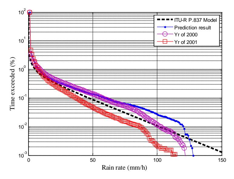
Figure 1 Percentage of time exceeded versus rain rate between measured and predicted data compared with the model of recommendation ITU-R P.837-5.
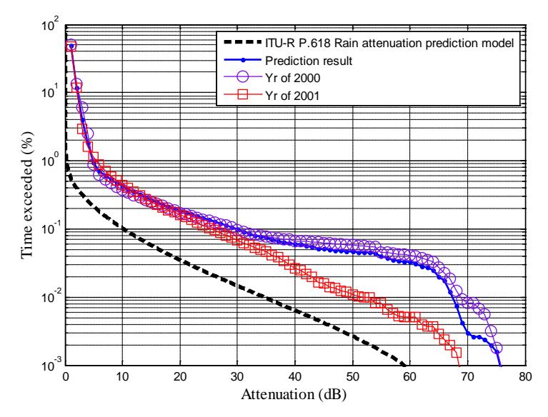
Figure 2 Percentage of time exceeded versus rain propagation attenuation between measured and predicted data compared with the model of recommendation ITU-R P.618-10.
3.2 Statistical Data of Measurement and Prediction Result
In general, the statistical characterization of rain is initiated by dividing the world into rain climate zones [12]. Within each zone, the maximum rain rate for a given probability is determined from actual meteorological data accumulated over many years. This is useful to assist engineers in designing satellite communications links, since it is unfeasible to guarantee performance under every possible condition. Hence, the system parameters are set to rational limits based on conditions that are expected to happen at a certain probability, while a fading margin is set to compensate for the effects of rain at a given level of availability. Table 1 and Table 2 show statistical data for measured and predicted rain rates, respectively. From Table 1, it can be noted that the higher the rain rate value, the less rain events occur. For 0.01% exceeded time in the years 2000 and 2001, the rain rate levels were 103 mm/h and 87 mm/h, respectively. When compared with the predicted rain rate in Table 2, the rain rate level for 0.01% exceeded time is higher, i.e. 115 mm/h. This happens since the HMM method implemented in the prediction used cumulative measured data from two years to obtain the HMM parameters, i.e. the transition and emission matrices, instead of data for one year (for either 2000 or 2001).
Table 1 Statistical data for measured rain rate.
| Rain | ≥10 | ≥20 | ≥30 | ≥40 | ≥50 | ≥60 | ≥70 | ≥80 | ≥90 | ≥100 | ≥110 | ≥120 | unit |
|---|---|---|---|---|---|---|---|---|---|---|---|---|---|
| rate | mm/h | mm/h | mm/h | mm/h | mm/h | mm/h | mm/h | mm/h | mm/h | mm/h | mm/h | mm/h | |
| 3625 | 1931 | 1283 | 865 | 595 | 385 | 267 | 181 | 95 | 48 | 29 | 8 | minutes | |
| 2000 | 0.824 | 0.439 | 0.292 | 0.197 | 0.135 | 0.088 | 0.061 | 0.041 | 0.022 | 0.011 | 0.007 | 0.002 | % |
| 2960 | 1228 | 676 | 367 | 208 | 126 | 83 | 57 | 30 | 9 | 7 | 2 | minutes | |
| 2001 | 0.6484 0.2690 0.1481 0.0804 0.0456 0.0276 0.0182 0.0125 0.0066 0.0020 0.0015 0.0004 | % | |||||||||||
| 6585 | 3159 | 1959 | 1232 | 803 | 511 | 350 | 238 | 125 | 57 | 36 | 10 | minutes | |
| Cum | 0.735 | 0.352 | 0.219 | 0.137 | 0.090 | 0.057 | 0.039 | 0.027 | 0.014 | 0.006 | 0.004 | 0.001 | % |
Table 2 Statistical data for predicted rain rate.
| Rain | ≥10 | ≥20 | ≥30 | ≥40 | ≥50 | ≥60 | ≥70 | ≥80 | ≥90 | ≥100 | ≥110 | ≥120 | unit |
|---|---|---|---|---|---|---|---|---|---|---|---|---|---|
| rate | mm/h | mm/h | mm/h | mm/h | mm/h | mm/h | mm/h | mm/h | mm/h | mm/h | mm/h | mm/h | |
| Pred | 3590 | 1964 | 1346 | 917 | 681 | 491 | 350 | 273 | 202 | 126 | 90 | 42 | minutes |
| 0.718 | 0.3928 0.2692 0.1834 0.1362 0.0982 0.07 0.0546 0.0404 0.0252 0.018 0.0084 | % |
Recommendation ITU-R P.1623-1 states that in the design of telecommunication systems, including satellite communications links, the dynamic characteristics of fading due to atmospheric propagation has to be considered to optimize system capacity and to accomplish the requirements of quality and reliability. Several temporal scales can be defined since it is useful to have information about fade duration and interfade duration statistics for a given attenuation level. Fade duration is defined as the time interval between two crossings above the same attenuation threshold, whereas interfade duration is the time interval between two crossings below the same attenuation threshold [11].
Table 3 Statistical data for measured rain propagation attenuation in the year 2000.
| Level threshold (dB) | |||||||||||
|---|---|---|---|---|---|---|---|---|---|---|---|
| 1 | 3 | 5 | 10 | 20 | 30 | 40 | 50 | 60 | 70 | ||
| Number of event above threshold (times) | 22375 | 4659 | 514 | 345 | 250 | 169 | 109 | 81 | 85 | 19 | |
| Average fade duration (minutes) | 2.91 | 2.60 | 7.11 | 6.18 | 4.23 | 3.62 | 4.18 | 4.91 | 3.36 | 1.89 | |
| Max fade duration (minutes) | 380 | 191 | 83 | 71 | 64 | 64 | 64 | 64 | 20 | 9 | |
| Standard deviation | 34.53 | 6.16 | 11.08 | 9.50 | 6.72 | 6.99 | 8.22 | 8.96 | 3.79 | 2.00 | |
| Number of event under threshold (times) | 22376 | 4660 | 515 | 346 | 251 | 170 | 110 | 82 | 86 | 20 | |
| Average interfade duration (minutes) | 20.65 | 110.50 1016.29 1517.08 2095.55 3096.64 4787.13 6422.46 6125.05 26350 | |||||||||
| Max interfade duration (minutes) | 4302 | 15297 | 43336 | 43341 | 54449 | 109705 113838 258013 258013 258015 | |||||
| Standard deviation | 96.07 | 699 | 3111 | 4051 | 5588.33 10139 | 14002 | 29108 | 28898 | 65976 | ||
Table 4 Statistical data for measured rain propagation attenuation in the year 2001.
| Level threshold (dB) | |||||||||||
|---|---|---|---|---|---|---|---|---|---|---|---|
| 1 | 3 | 5 | 10 | 20 | 30 | 40 | 50 | 60 | 70 | ||
| Number of event above threshold (times) | 24452 | 1505 | 661 | 316 | 186 | 124 | 77 | 37 | 21 | 5 | |
| Average fade duration (minutes) | 2.26 | 5.4 | 6.61 | 6.39 | 4.31 | 2.78 | 1.84 | 1.62 | 1.38 | 1 | |
| Max fade duration (minutes) | 181 | 88 | 67 | 62 | 33 | 16 | 7 | 6 | 6 | 1 | |
| Standard deviation | 5.82 | 10.34 | 10.16 | 8.58 | 5.2 | 2.53 | 1.35 | 1.16 | 1.12 | 0 | |
| Number of event under threshold (times) | 24453 | 1506 | 662 | 317 | 187 | 125 | 78 | 38 | 22 | 6 | |
| Average interfade duration (minutes) | 19.23 | 344 | 787.35 | 1652 | 2806 | 4202 | 6737 | 13830 | 23890 | 87599 | |
| Max interfade duration (minutes) | 9890 | 12784 | 18289 | 18439 | 28853 | 63841 | 67480 147137 161281 444158 | ||||
| Standard deviation | 3.51 | 16.58 | 25.16 | 25.47 | 32.92 | 37.82 | 41.32 | 22.65 | 15.7 | 0 | |
The statistical data for measured rain propagation attenuation in the years 2000 and 2001 are summarized in Table 3 and Table 4, respectively. These tables show the distribution of statistical parameters such as the number of events for fade duration, the average fade duration, the number of events for interfade duration, the average interfade duration, etc. It seems that the measured data for the year 2000 and those for 2001 are similar. For comparison, the statistical data for predicted rain propagation attenuation are tabulated in Table 5. Note that the statistical data of the predicted results are identical to the measured results from Table 3 and Table 4. A significant discrepancy between the measured and the predicted data is only seen in the standard deviation for fade duration and interfade duration. This occurs because statistical parameters show only the distribution, not a time series, which evokes the discrepancy in standard deviation.
| Level threshold (dB) | |||||||||||
|---|---|---|---|---|---|---|---|---|---|---|---|
| 1 | 3 | 5 | 10 | 20 | 30 | 40 | 50 | 60 | 70 | ||
| Number of event | |||||||||||
| above threshold (times) | 46474 | 7574 | 2626 | 1305 | 598 | 342 | 240 | 195 | 129 | 12 | |
| Average fade duration (minutes) | 1.22 | 1.23 | 1.37 | 1.46 | 1.45 | 1.33 | 1.23 | 1.17 | 1.19 | 1.08 | |
| Max fade duration (minutes) | 68 | 62 | 61 | 46 | 29 | 14 | 7 | 7 | 7 | 2 | |
| Standard deviation | 1.07 | 1.46 | 2.08 | 2.42 | 1.74 | 1.11 | 0.63 | 0.60 | 0.69 | 0.29 | |
| Number of event under threshold (times) | 46475 | 7575 | 2627 | 1306 | 599 | 343 | 241 | 196 | 130 | 13 | |
| Average interfade duration (minutes) | 9.54 | 64.78 | 188.96 | 381.39 | 833.28 1456.40 2073.46 2549.85 3844.98 38461 | ||||||
| Max interfade duration (minutes) | 98 | 541 | 1807 | 3906 | 6184 | 19389 | 19406 | 28640 | 28640 | 75469 | |
| Standard deviation | 9.35 | 72.92 | 245.16 | 475.80 | 1028 | 2133.88 | 2915 | 3660 | 5236 | 28348 | |
Table 5 Statistical data for predicted rain propagation attenuation.
4 Conclusion
The rain rate and rain propagation attenuation for K-band satellite communications links based on measurement data in tropical areas have been successfully predicted using the HMM method. The predicted rain rate had similarity with the measured data as well as with the model of recommendation ITU-R P.837-5 for low rain rates. However, it was different for high rain rates. For rain propagation attenuation, the model of recommendation ITU-R P.618- 10 for rain propagation attenuation has not given good results compared to the prediction method based on HMM. The predicted rain propagation attenuation showed a good agreement with the measured data. From statistical data obtained using the model of recommendation ITU-R P.1623-1, such as fade duration and interfade duration, it can be seen that the discrepancy between the measured and the predicted data was insignificant. In addition, further investigation into mitigation techniques for rain attenuation propagation can be proposed by implementing the proposed method to predict the attenuation for a short time period so that mitigation can be set adaptively.
Acknowledgements
This work uses measured data from a co-operation between ITB, Indonesia, and JAXA (NASDA) and NiCT (CRL), Japan, in the PARTNERS (Pan Asia Pacific Region Telecommunication Network for Experiments and Research by Satellite) project.