
1 0BIntroduction
Monitoring activities that occur in a computer system or network and analyzing them to recognize signs of an attack, identifying it as an attempt that endangers confidentiality, integrity and availability of the computer system or network or breaks through the security mechanism, is known as intrusion detection [1]. Signature-based detection capabilities rely on attack pattern information that has been collected in a database. A deficiency of this method lies in the inability to detect new patterns that do not exist in the database. Anomaly detection uses a history of normal patterns and detects deviations from these patterns.
Intrusion detection systems (IDS) can run in real-time or offline, using a centralized or distributed architecture. Centralized architectures are widely used to identify attacks on a single system that is being monitored. Distributed and coordinated attacks, such as DDoS, using many machines as attackers or victims, are likely to increase. Analysis based only one source location has difficulty to identify this type of attack. To overcome this, a distributed intrusion detection system (DIDS) is needed.
Problems on attack detection can be reduced to problems of classification and clustering. Methods that have been developed in the direction of its application provide high quality results quickly and efficiently [2]. A clustering algorithm can be based on partitional or hierarchical clustering. Basic partitional clustering algorithms have a linear running time and some are able to handle large amounts of data, such as k-means clustering, but they still have shortcomings in terms of dependence on initial conditions and the results of initiation tending towards a local minimum [3].
Swarm intelligence techniques aim to solve complicated problems through the development of simple agents working together without supervision to achieve the optimal solution through a mechanism of direct or indirect communication, where agents are constantly exploring the search space. The agents are used to complete the difficult task of finding the classification rules for signature-based detection and finding clusters for anomaly-based detection. They have the ability to organize themselves (self-organization), which is used to divide the problem into simpler subproblems that are given to different agents. This capability has the potential to make the IDS autonomous, able to adapt, parallel, self-organized and efficient [2].
The ant colony clustering (ACC) algorithm from the field of swarm intelligence, inspired by ant-colony intelligence, is a Lumer-Faieta (LF) model that combines hierarchical-based and partitional-based clustering without requiring initiation of the number of clusters. In hierarchical clustering, the object is initially regarded as a cluster and it is iteratively merged through a comparison of attributes to assess dissimilarity. In partitional clustering (a) the object comparisons are made with the mean (centroid) in the cluster, and (b) cluster membership can be moved [4].
ACC was inspired by two behaviors of ant colonies, firstly brood care performed by the colony, each individual ant working independently without receiving orders from others in a higher hierarchical position. For example, in the nest, the eggs, larvae and food are not scattered around randomly, but follow spatial patterns. Secondly, the behavior of cemetery organization with which the colony deals with dead members. Each individual ant shows funereal
behavior by randomly moving around to collect the remains of dead ants and arrange them in the form of clusters. Both of these behaviors are based on the ability of ants to compare objects that are encountered when exploring the search space [4].
Two major problems in the development of an ACC-based IDS are the algorithmic aspect of detection (computational) and the communication between components of detection (architectural). From the computational point of view, the ability of novel-attack detection is lacking, detection rate (DR) and false alarm rate (FAR) are not ideal, large data traffic leads to burdensome computation, detection through real-time data analysis while a session is running and immediate alarm notification are difficult. Issues from the architectural point of view are: difficulty to overcome distributed and coordinated attacks because this requires large amounts of distributed information, the synchronization of information between distributed components of detection is difficult, the network traffic due to the distribution of large amounts of information between components is burdening, cooperation between components of detection is lacking, and the centralized hierarchical structure between components allows attackers to cut off the lines of communication and command the central node.
The aim of this research was to develop an architecture of distributed IDS that implements an ACC detection algorithm that is able to recognize new attacks and coordinated attacks, handle huge data and traffic, has synchronization capabilities, has the ability of cooperation between components without the presence of centralized computing components, execute detection in real-time and send an alarm notification immediately.
2 Related Work
ACC has evolved into two different directions, namely models without communication mechanism and models using indirect communication. Pheromones are used in the communication mechanisms of ant colonies in search for food sources to determine the shortest path toward a food source (foraging behavior). ACC models in the first group include: (a) basic models [5], (b) Lumer-Faieta (LF) models [6] and (c) ATTA models [7]. The second group uses pheromones as communication mechanism, for example: (a) ANTIDS models [8], (b) ACCM models [9], (c) hybrid ACC and C4.5 models [10], and (d) ACCA-IDS models [11].
2.1 ACC without Direct Communication
The ACC basic model (BM) was first proposed by Deneubourg, et al. [5] and applied in so-called ant-like robots (ALR) or robot-like ants (RLA), performing simulation of ant behavior in clustering and sorting objects. A number of robots moves around randomly, without direct communication with each other, without having any hierarchy in their organization and without knowing any global mapping. They are only able to see objects in front of them and to distinguish between two or more different types of objects with a certain error rate [5].
The assumptions of BM were: (a) all objects and RLAs are placed randomly in a 2D grid space, (b) only one object can be placed in one position of the grid, (c) RLAs randomly move one step at each iteration (Figure 1).
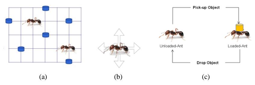
Figure 1 (a) 2D grid space for ants and objects placed randomly at the first iteration (b) four possible directions for ants moving randomly, and (c) conditions for an ant to pick up an object it found or dropping the object it was carrying.
If at some location there is an object as well as an RLA in unloaded condition, then the probability of the RLA taking the object is: \(P_{pick} = \left[\frac{k_{pick}}{k_{pick}+\lambda}\right]^2\), where \(\lambda\) is the proportion of the number of objects (n) found by the RLA at the T last steps. T is determined using the short-term memory (m) of the RLA. For example, if m=3 is the short-term memory at the \(5^{th}\) step (10111), then n is determined only at the three last steps (111) of the 5 steps that have been taken by the RLA. In loaded condition, the probability of the RLA dropping the object at a given location is: \(P_{drop} = \left[\frac{\lambda}{k_{drop} + \lambda}\right]^2\), where \(k_{pick}\) is a constant value for \(p_{pick}\) and \(k_{drop}\) for
\(p_{drop}\).
The Lumer-Faieta (LF) model is a modified BM making it able to handle numerical data, improving the quality of solutions and the convergence time [12]. Its function f(i) (1), which identifies conditions in the environment using the dissimilarity between individuals data \(\delta(i,j)\), is defined as:
\[f(i) = \begin{cases} \frac{1}{\sigma^2} \sum_{j} \left( 1 - \frac{\delta(i,j)}{\alpha} \right), & \text{if } f(i) > 0\\ 0, & \text{otherwise} \end{cases}\] (1)
where \(\delta(i,j)\) is the dissimilarity function between objects \(o_i\) and \(o_j\) in the data space using the Euclidian distance, \(\alpha \in [0,1]\) is a scaling parameter of the data, and \(\sigma' \in \{9,25\}\) is the size of the local environment around the RLA. The environment around the RLA is a square grid, so the radius of perception (\(\sigma\)) is \(\frac{\sigma-1}{2}\). While moving randomly in the 2D grid, the unloaded-RLA decides to take action (pick up or drop \(o_i\)) when it finds an object \(o_i\) in a location, using the average similarity between \(o_i\) and all \(o_j\) in local environment \(\sigma'\) (Figure 2). Thus f(i) aggregates the RLA's environment, where empty locations will not contribute to the function.
Figure 2 An ant in a 2D-grid space finds an object \(o_i\) at a position, then moves using the average similarity between \(o_i\) and all \(o_i\) in local environment \(\sigma = 3\).
Short-term memory for keeping information about the location of the last dropped object was also introduced in LF. After picking up \(o_i\), it compares dissimilarity \(\delta(i,j)\) between \(o_i\) and \(o_j\) in its memory, chooses the most similar one and then jumps to the location of \(o_j\). LF also introduced non-homogeneous colonies using velocity v to distinguish slower RLAs that are more selective in performing the pick up or drop action and fast-moving RLAs that form clusters.
There are shortcomings of the LF model in terms of convergence. While the number of data increases, the clustering process produces many small clusters of similar objects that are not visible and will be merged with enough computing time. LF proposed a switching behavioral mechanism for the RLAs to change the behavior of building clusters into destroying clusters during phases of stagnancy [12].
The adaptive time-dependent transporter ants (ATTA) model [12] proposes two modifications for function f(i). Firstly, an empty location or loose cluster will not contribute to the function other than locations filled with an object or dense clusters, and secondly it uses the restriction of \(\forall_j \left(1 - \frac{\delta(i,j)}{\alpha}\right) > 0\) for the case of high dissimilarity leading to spatial separation between clusters in the 2D
grid space. Four other changes are also included in ATTA. Firstly, too many idle phases because of objects not being found while the RLAs move around randomly (in BM and LF) causes a significant increase in iterations, so eager ants were introduced. The RLA contributes to the clustering process when it finds oi on the grid. It is then set to go to the location of another object for picking it up directly. Secondly, ATTA also uses jump ants. If the step size value is large in LF, the RLA is able to jump directly to another location that contains a small cluster of objects of the same type to be merged, resulting in a time reduction of the iteration process. Thirdly, α-adaptation was introduced as an adaptation scheme of α in order to cluster data. And fourthly, control of stagnation was introduced to avoid blockage by RLAs dropping the object they carry because of outlier values in the data. If the iteration number is high and the RLA does not drop the object, then it drops deterministically [12].
2.2 ACC with Indirect Communication Using Pheromones
Investigation of an ACC-based IDS using pheromone mechanisms for indirect communication was first conducted by Ramos and Abraham through the ANTIDS model [8], by Tsang and Kwong through the ACCM model [9],[13], a hybrid model through ACC and C4.5 [10], and the ACCA-IDS model [11]. ANTIDS proposed an algorithm similar to the algorithm of LF against the KDD1999 dataset. ACCM featured several improvements of LF.
| Attack | Winner on | K-Means Clustering [14] | ACC-Based IDS using KDD1999 | ||||
|---|---|---|---|---|---|---|---|
| Category on KDD1999 | KDD1999 [14] | ANTIDS [8] | ACCM [9] | ACC-C4.5 [10] | ACCA-IDS [11] | ||
| Normal | 99.50 | 96.20 | 99.73 | 98.80 | 95.42 | - | |
| Probe | 83.30 | 86.90 | 99.86 | 87.50 | 99.70 | 99.40 | |
| DoS | 97.10 | 94.20 | 99.97 | 97.30 | 99.35 | 99.20 | |
| U2R | 13.20 | 27.40 | 68.00 | 30.70 | 73.20 | 99.70 | |
| R2L | 8.40 | 6.50 | 99.47 | 12.60 | 71.10 | 99.50 | |
Table 1 Detection accuracy (%) between ACC-Based IDS using KDD1999.
Detection accuracy of ANTIDS and ACCM was tested on KDD1999, showing results beyond the k-means winner on KDD1999 (Table 1), especially in userto-root (U2R) and remote-to-local (R2L) attacks that appeared in the testing dataset compared to the training dataset. This shows that methods based on colony intelligence, such as ACC, are adaptive and are able to recognize new types of attacks more easily.
Some of the advantages offered by ANTIDS (ANT colony-based IDS) [8]: detection is done online and in real-time because it is distributed. In contrast, DT, SVM, LGP and SOM are not able to classify new data or new categories and visualize them continuously or in a self-organized way. Also, repetition of the learning process is done from the beginning. Handling new classes can be done without retraining. The stigmergy mechanism in the colony is relevant to aspects of flexibility when environmental changes occur due to interference from outside of the system, so members of the colony can respond appropriately to disturbances as if environmental modifications are made by the ants collectively, using the same behavior. A colony is able to work either unsupervised or supervised by adding classification results using k-NNR and marking them using the training data. ANTIDS self-organized nature makes it a potential distributed IDS.
According to Tsang and Kwong [13], large and high dimension data are known as a feature of IDSs. There are two inefficiencies in LF. First, a number of homogeneous clusters is formed that are difficult to combine when they are separated in a large search area. Second, it measures the intensity of an object's similarity, directs the formation of clusters in dense areas locally but also distinguishes objects that are not intensively similar. Therefore, object A and object B which are close to a dense cluster, will tend to remain isolated and separated [13]. Hence, the authors proposed the ant colony clustering model (ACCM), which combines local entropy and the average similarity of objects to identify clusters as "coarse", "dense" and "not suitable", and then merges them into a single cluster. Two types of pheromones, the object and cluster pheromone, guide loaded ants towards a cluster position and unloaded ants to an position of an isolated object in a certain area [9]. ACCM also offers an initial architecture based on IDS using multi-agents [14].
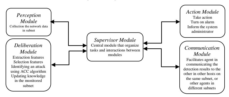
Figure 3 Architecture of agents in a node [15].
We use an agent architecture consisting of several modules (Figure 3) [15], namely: (1) the perception module (PM), which is responsible for audit and network data collection in subnets where the agent is located; (2) the deliberation module (DM), which is responsible for the extraction and selection of features that are collected by the PM so that the agent can perform the task of recognizing an attack using the ACC algorithm and updating knowledge in the monitored subnet; (3) the communication module (CM), which facilitates the agent in communicating the detection results to other agents on the same subnet or other agents in different subnets; (4) the action module (AM), which takes appropriate steps when an attack is successfully recognized and reaches the threshold of an attack; it will send an alert and communicate it to the system administrator; (5) the supervisor module (SM), which is responsible as the central module that organizes tasks and interactions between modules.
We also use 3 types of agents and the ways they communicate with each other (Figure 4) [15] by adding ACC engine as knowledge basis for detecting an intrusion. First, the supervisory agent system (SAS), which is assigned to collect, prepare and disseminate attack specification data; when there is demand it immediately implements the data collection process. Second, supervisory agent attacks (SAA), which utilizes the data released by SAS and other SAAs. Each SAA uses an ACC algorithm to build attack knowledge (cluster models) in order to recognize an attack on the host and then updates the knowledge about attacks that have been built utilizing data from other SAAs. Third, the agent register (AR), which manages the registry of every SAS and SAA for the management of controlled variables and uses it to find the name and location of other agents and the data of interest of other agents using the interest mechanism.
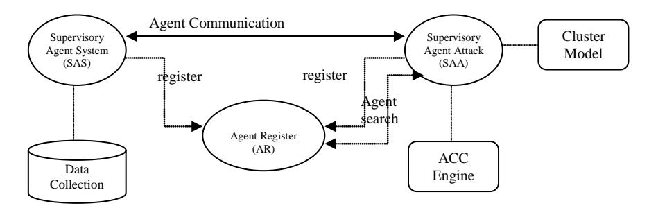
Figure 4 Communication between supervisory agent system (SAS) and supervisory agent attacks (SAA) through agent register (AR) [15].
2.3 Developing Single IDS into Distributed IDS
At first, IDSs were placed in a single host (host-based IDS). They monitored the operating system logs and performed simple pattern matching to a small set of signatures [16]. The sensor and detector components of a host-based IDS are placed in the same host. Then the attacks developed, as well as the components of detectors and detection methods. Networking technologies were developed that make data location distributed over networks, as well as sensors that transmit data to a central node and perform a centralized hierarchical detection method, the so-called host-based IDS using distributed sensors.
Sending large volumes of data and high complexity sensor data to the centralized node may leave the door open and cause vulnerability of the huge amount of network data and the system itself. Hence, IDS evolved into distributed IDS (DIDS), meaning the detectors as well as the sensors are distributedly placed over a network but still in a centralized hierarchy. Our proposed architecture consisting of multi-agents is shown in Figure 5.
Figure 5 Illustration of our proposed agents in a network.
2.4 Selecting Features Based on PCA
Principal component analysis (PCA), also called Hotelling transformation, is a classical technique in statistics for data analysis, feature extraction and data reduction [17]. PCA performs a linear combination of correlated features, transforms them into a lower dimensional space and makes them uncorrelated. Highly correlated data indicate information redundancy, so PCA will reduce the redundancy by removing correlations and minimize information loss due to the decrease in size. This means that PCA is able to transform and reduce the initial features' dimension while maintaining a maximum of original information and identifying the structure of relationships between variables that contribute predominantly to the variable transformation results.
The process of singular value decomposition (SVD) can be made into a correlation matrix S for the determination of the eigenvalues (λi) in diagonal
matrix \(\Lambda\) and eigenvectors in matrix \(\mathbf{U}\). Diagonal matrix \(\Lambda\) values on the diagonal are eigenvalues \(\lambda_i\) (for i=1,2,...p). Eigenvalues \(\lambda_i\) are the variance for each direction indicated by the eigenvectors \(u_i\), while \(\lambda_I\) is the maximum variance direction indicated by the eigenvectors \(u_I\). The eigenvectors form the new axes (dimensions) of the new feature. The dimensional reduction from the initial dimension of standardized value \(ZX_i\) creates a new dimension k, where k < p, using a percentage of variance explained by each eigenvalue determined by \(c_i = \frac{\lambda_i}{\sum_{i=1}^{k} \lambda_i}\). k is determined by using: (a) the Kaiser criteria by looking at eigenvalues \(\geq 1\), (b) the decrease of the value of \(c_i\) in scree plot which is quite steep and (c) any other important aspects related to the intended use.
3 Methodology
3.1 NSL-KDD Dataset
In the evaluation study of IDS, the NSL-KDD dataset was the standard benchmark [18] as an improvement of dataset KDD1999. It is widely used in anomaly detection [19]. The data were produced by processing the tcpdump of the DARPA1998 IDS evaluation data from the MIT Lincoln Laboratory under DARPA sponsorship [20]. NSL-KDD consists of 43 variables that are classified into basic features, content and traffic (Table 2).
KDDTrain+ and KDDTest+ as subsets of NSL-KDD were prepared as a source of data for preparation, analysis and testing. Preparation consisted of the following steps: (a) selecting normal activity and probing activity (nmap, ipsweep, portsweep, and satan) from KDDTrain+ for training data; (b) selecting normal activity and probing activity (nmap, ipsweep, portsweep, satan, and added two new probing activities, saint and mscan) of KDDTest+ for data testing; and (c) selecting features in KDDTrain+ and KDDTest+.
The analysis stage utilized KDDTrain+NP and performed the following steps: (a) standardizing the values of the features; (b) performing data exploration to assess the feasibility of assumptions such as the relationship between variables and the nature of the identity correlation matrix; (c) extracting the correlation matrix and its singularity; (d) analyzing the diversity of the data (univariate and multivariate) to see differences in the characteristics of the objects observed (normal and probing activity); (e) performing PCA to reduce high dimension of data, determining the main components or factors (FAC), and determining the dominant variables in each factor; (f) identifying the grouping variable to study the characteristics of the probing activity and create a new data subset by grouping results; (g) selecting the subset for testing purposes.
Table 2 Features list in the dataset NSL-KDD.
| Feature | Description | Тур | |
|---|---|---|---|
| X1 duration | length (number of seconds) of the connection | С | |
| X2 protocol_type | . P. Q. | type of the protocol, e.g. tcp, udp, etc. | D |
| X3 service | Basic features of individual TCP connections | network service on the destination, e.g., http, telnet, etc. | D |
| X4 flag | atu ual :cti | number of data bytes from source to destination | C |
| X5 src_bytes | c fe vid | number of data bytes from destination to source | C D |
| X6 dst_bytes X7 land | asie ndi | normal or error status of the connection 1 if connection is from/to the same host/port; 0 otherwise | D D |
| X8 wrong_fragment | E. B | number of "wrong" fragments | C |
| X9 urgent | number of urgent packets | C | |
| X10 hot | number of ``hot" indicators | C | |
| X11 num_failed_logins | number of failed login attempts | C | |
| X11 hum_juueu_logins X12 logged_in | 1 if successfully logged in; 0 otherwise | D | |
| z | C | ||
| X13 num_compromised | Content features within a connection | number of ``compromised" conditions | |
| X14 root_shell | atu ne | 1 if root shell is obtained; 0 otherwise | D |
| X15 su_attempted | e fe | 1 if ``su root" command attempted; 0 otherwise | D |
| X16 num_root | a c | number of ``root" accesses | C |
| X17 num_file_creations | ond hin | number of file creation operations | C |
| X18 num_shells | wit. | number of shell prompts | C |
| X19 num_access_files | number of operations on access control files | C | |
| X20 num_outbound_cmds | number of outbound commands in an ftp session | C | |
| X21 is_hot_login | 1 if the login belongs to the ``hot" list; 0 otherwise | D | |
| X22 is_guest_login | 1 if the login is a ``guest"login; 0 otherwise | D | |
| X23 count | secor | number of connections to the same host (IP) as the current connection in the past two seconds | С |
| X24 srv_count | a two | number of connections to the same service (port) and same host (IP) as the current connection in the past two seconds | С |
| X25 serror_rate | using w affic) | % of connections that have ``SYN" errors to the same host during aggregation on X23 | C |
| X26 srv_serror_rate | computed usi time window 1e-based trafi | \(\%\) of connections that have ``SYN" errors to the \({\bf same}\ {\bf service}\ {\bf during}\ {\bf aggregation}\ {\bf on}\ X24\) | C |
| X27 rerror_rate | es computed using time window (time-based traffic) | % of connections that have ``REJ" errors to the same host during aggregation on X23 | C |
| X28 srv_rerror_rate | Iraffic features computed using a two-secon time window (time-based traffic) | % of connections that have ``REJ" errors to the same service during aggregation on X24 | C |
| X29 same_srv_rate | c fe | % of connections to the same service and the same host during aggregation on X23 | C |
| X30 diff_srv_rate | i£i. | % of connections to different services and the same host during aggregation on X23 | С |
| X31 srv_diff_host_rate | Tre | % of connections to different hosts and the same service during aggregation on X24 | C |
| X32 dst_host_count | number of connections to the same host (IP) in the last hundred connection | C | |
| X33 dst_host_srv_count | number of connections to the same service (port) in the last hundred connection | C | |
| X34 dst_host_same_ | C | ||
| srv_rate | 00 | % of connections to the same service and the same host during aggregation on X32 | C |
| usi do ic) | 0/ of compositions to different convices and the same heat during accordation on V22 | C | |
| X35 dst_host_diff_srv_rate | ed vin affi | % of connections to different services and the same host during aggregation on X32 | C |
| X36 dst_host_same_ | in the | % of connections from the same service during aggregation on X33 | C |
| src_port_rate | rmp ctio sed | ||
| X37 dst_host_srv_diff_ host_rate | res co onne on-bas | % of connections to different hosts during aggregation on X33 | С |
| X38 dst_host_serror_rate | ic features computed using ndred connection window nnection-based traffic) | % of connections that have ``SYN" errors to the same host during aggregation on X32 | С |
| X39 dst_host_srv_ serror_rate | Traffic a hun (con | \(\%\) of connections that have ``SYN" errors to the \(\mathbf{same}\) \(\mathbf{service}\) during aggregation on \(X33\) | С |
| X40 dst_host_rerror_rate | % of connections that have ``REJ" errors to the same host during aggregation on X32 | C | |
| X41 dst_host_ srv_error_rate | % of connections that have ``REJ" errors to the same service during aggregation on X33 | C | |
| Y1 attack_type | Label | DoS attack (back,land, neptune, pod, smurf, teardrop), Probe attack (ipsweep, nmap, | D |
| 11 иниск_куре | Lavei | portsweep, satan), R2L attack (ftp_write, guess_passwd, imap, multihop, phf, spy), |
4 Experiment Results and Analysis
4.1 Selecting Features Based on PCA
KDDTrain+ and KDDTest+ are subsets of NSL-KDD containing normal activities and nmap, ipsweep, portsweep, and satan probing activities. The KDDTrain+ subset contained 78.999 row data, consisting of 67.343 normal activities (85.25%) and 11.656 probing activities (14.75%), and was subsequently called KDDTrain+NP, with a ratio of 5:1 between normal and probing activities. KDDTest+NP was prepared for testing purposes, containing normal activities and nmap, ipsweep, portsweep, and satan probing activities, and two new types of probing were added that were not contained in KDDTrain+NP, namely mscan and saint. It contained 12.132 row data, consisting of 9.711 normal (80%) and 2.421 probing activities (20%).
All 78.999 data in KDDTrain+NP had 32 features with numerical variables. There were two features that did not have variablity in value, i.e. wrong_fragment (X8), which indicates the number of packets containing a bad checksum in each of the connections, and num_outbound_cmds (X20), which indicates the number of orders outside the network segment (outbound) in an FTP session. Meanwhile in KDDTest+NP, which contained 12.132 activities, there were three features that had no variance: urgent (X9), num_shell (X18) and num_outbound_cmds (X20). The no-variance condition excluded these features from further processing.
Statistical values show the use of different scales on these features. The next stage calculates the ZXij value by subtracting each observation Xij with the average xi and then divides the result by their standard deviation (si). This standardization will produce transformation data that have a distribution of values between -1 to 1 and are centered around a value of 0. This process is expected to show a pattern of differences between normal and probing activities. An average value and a very high diversity were seen in some features, such as X1 (duration), X5 (src_bytes), and X6 (dst_bytes). Descriptive statistics of 28 standardized values showed an average value of 0 and standard deviation 1. Although 28 features had a size and spread of the same concentration, they still had a different range in sizes.
4.1.1 Dimensional Reduction
Most correlations between ZXi and ZXj (for i ≠ j) showed significant values in correlation matrix S. The values of the partial correlation coefficient indicated a partial linkage between some of the features. Small values or values close to zero can cause S to become an identity matrix with the one diagonal is 1, while the other is zero, so we tested under null hypothesis how small those values were. The Kaiser-Meyer-Olkin (KMO) test under null hypothesis verifies how small the correlation coefficient in matrix S is and the Bartlett test under null hypothesis verifies if S is an identity matrix. These two tests showed a significance level of 0. It showed empirically that no null hypothesis was true and that the correlation coefficient cannot be regarded as small and S was not an identity matrix.
Rejection of the null hypothesis means that PCA is suitable for transforming and reducing the initial dimension, while maintaining a maximum of original information and can identify the structure of relationships between variables that contribute predominantly to the variable transformation results. The SVD process of correlation matrix S resulted 28 eigenvalues (\(\lambda_i\)). The value of \(\lambda_i\) is the variance for each direction indicated by the eigenvectors \(u_i\) and the first eigenvalue \(\lambda_I\) is the maximum variance direction indicated by the first eigenvector \(u_I\). The eigenvector form the new features or axes (dimensions) that are called by a factor (FAC). Table 3 shows all 28 eigenvalues (\(\lambda_i\)).
| i | \(\lambda_i\) | ci (%) | % Cum. | \(i\) \(\lambda_i\) | \(c_i\) \((\%)\) | % Cum. | \(i\) \(\lambda_i\) | ci (%) | % Cum. |
|---|---|---|---|---|---|---|---|---|---|
| 1 | 5.769 | 20.605 | 20.605 | 10 1.000 | 3.570 | 74.078 | 20 0.376 | 1.342 | 97.368 |
| 2 | 2.881 | 10.289 | 30.893 | 11 0.994 | 3.552 | 77.630 | 21 0.193 | 0.689 | 98.057 |
| 3 | 2.437 | 8.703 | 39.596 | 12 0.985 | 3.517 | 81.147 | 22 0.162 | 0.578 | 98.635 |
| 4 | 2.176 | 7.771 | 47.367 | 13 0.791 | 2.824 | 83.970 | 23 0.123 | 0.438 | 99.073 |
| 5 | 1.740 | 6.213 | 53.580 | 14 0.739 | 2.638 | 86.608 | 24 0.096 | 0.343 | 99.416 |
| 6 | 1.441 | 5.147 | 58.727 | 15 0.722 | 2.580 | 89.189 | 25 0.084 | 0.300 | 99.715 |
| 7 | 1.258 | 4.494 | 63.221 | 16 0.561 | 2.005 | 91.193 | 26 0.066 | 0.237 | 99.952 |
| 8 | 1.038 | 3.706 | 66.927 | 17 0.475 | 1.696 | 92.889 | 27 0.013 | 0.045 | 99.997 |
| 9 | 1.003 | 3.582 | 70.509 | 18 0.454 | 1.622 | 94.511 | 28 0.001 | 0.003 | 100.000 |
| 19 0.424 | 1.515 | 96.026 |
Table 3 List of 28 eigenvalues.
The dimensional reduction process from p=28 (\(ZX_i\)) creates a new dimension k<28 using percentage of variance, explained by each eigenvalue determined by \(c_i = \frac{\lambda_i}{28}\). Using the Kaiser criteria eigenvalues \(\geq 1\) and looking at the decreased value of \(c_i\) in scree plot, a value of k = 14 (50% reduction) is selected. The eigenvalues \(\lambda_i\) (for i = 1,2, ... 14) and the cumulative percentage of variance can be extracted from the initial data's \(ZX_i\) of 86.61%.
4.1.2 Relationship between Initial and New Features from PCA
The component matrix of factor loadings consists of coefficients in the eigenvector that indicate the direction of the axis on the new dimension (FAC) and are affected by the values of \(ZX_i\). For example, for the first eigenvector \((u_I)\)
as an FAC_1 axis the coefficient of ZX27, ZX28, ZX35, ZX40 and ZX41 is large enough (more than 0.7) or small enough (ZX34 less than -0.7). Eigenvector u1 can be said to be influenced by ZX27, ZX28, ZX35, ZX40 and ZX41 which have a positive effect (increase), and ZX34, which has a negative influence (reduce). The relationship reveals a hidden factor that is influenced by the initial features in the original dimensional space. The relationship between the initial features ZXi and factor (FAC) is shown in Table 4.
The relationship can be either positive or negative. FAC_1 is positively associated with features such as rerror_rate, srv_rerror_rate, dst_host_diff_srv_rate, dst_host_rerror_rate and dst_host_srv_rerror_rate. Negative association occurs between FAC_1 and dst_host_same_srv_rate. FAC_1 seems a representation of SYN error and REJ error when connecting to the same IP and destination port, and to the same IP on different services.
Table 4 Relationship between ZXi with factors (FAC).
| Factor | Positive Effects (loading ≥ 0.7) | Related Features | Negative Effects (loading ≤ -0.7) | Related Features | Interpretation of Factor |
|---|---|---|---|---|---|
| FAC_1 | ZX27 | rerror_rate | ZX34 | dst_hos | SYN error and REJ error |
| ZX28 | srv_rerror_rate | t_ | factor when connecting | ||
| ZX35 | dst_host_diff_ | same_s | to the same IP and the | ||
| srv_rate | rv_rate | destination port and | |||
| ZX40 | dst_host_ rerror_rate | connections to the same | |||
| dst_host_srv_ | IP on different services | ||||
| ZX41 | rerror_rate | ||||
| FAC_2 | ZX25 | serror_rate | - | SYN error factor when | |
| ZX26 | sev_serror_rate | the connection to the IP | |||
| ZX39 | dst_host_srv_serror_r | and port number the same | |||
| ate | purpose in time | ||||
| windowing 2 seconds and | |||||
| the connection | |||||
| windowing 100 | |||||
| connections | |||||
| FAC_4 | ZX13 | num_compromised | - | the emergence of a factor | |
| ZX16 | num_root | "not found" error and the | |||
| operation as root | |||||
| FAC_8 | ZX17 | num_file_creations | - | factors that created the | |
| file | |||||
| FAC_9 | ZX5 | src_bytes | - | factor data (bytes) sent | |
| from the IP source when | |||||
| the connection takes | |||||
| place | |||||
| FAC_10 | ZX6 | dst_bytes | - | factor of data (bytes) | |
| received during the | |||||
| connection | |||||
| FAC_11 | ZX11 | num_failed_login | factor that related to the | ||
| error log occur when the | |||||
| connection | |||||
| FAC_13 | ZX19 | num_access_files | - | factor controlling the | |
| files when the connection | |||||
| takes place |
The relation between FAC_2 with serror_rate, sev_serror_rate, and dst_host_srv_serror_rate shows a representation of SYN error when connecting to the same IP and port number in 2 seconds of time-windowing and 100 connections of connection-windowing. FAC_4 is closely associated with num_root and num_compromised, which indicates the emergence of a "not found" error factor and the operation as root. FAC_8 related with num_file_creations shows the presence of a factor that created a file. The relation between FAC_9 with src_bytes indicates the presence of data (bytes) sent from the IP source when the connection takes place. FAC_10 associated with dst_bytes shows a factor of data (bytes) received during the connection. The relation between FAC_11 with num_failed_login shows the presence of a factor that is related to the error log occuring when the connection takes place. Meanwhile, FAC_13 associated with num_access_files indicates the presence of a factor controlling the files when the connection takes place. Extraction FACij scores for each value of ZXij observations is performed using a regression method and produces a major component score coefficient matrix. A single value score is a representation of an observation on the new dimension.
4.1.3 New Features Characteristics
Using the score values, further testing was performed to see the differences between the two types of activities in the new dimension. This revealed some interesting patterns. The average value of normal activities had a negative sign (≤ 0), as opposed to probing activities, which had a positive sign (≥ 0) on FAC_1, FAC_3, FAC_6, FAC_7, FAC_9, FAC_13 and FAC_14. The opposite occured in dimension FAC_2, FAC_4, FAC_5, FAC_8, FAC_10, FAC_11, and FAC_12, seeing the value of the average normal activity was positive, while compared the average value of probing activities was marked otherwise. This
| Table 5 | Two groups of new features based on different signs class average. |
|---|
| Normal | Probe | t-Test | |||
|---|---|---|---|---|---|
| Subset | New Features | Average | Average | Significant | |
| Subset1 | FAC_1 | -0.2513 | 1.4518 | 0.0000 | |
| FAC_3 | -0.1254 | 0.7242 | 0.0079** | ||
| FAC_6 | -0.1188 | 0.6862 | 0.0000 | ||
| FAC_7 | -0.0870 | 0.5024 | 0.0000 | ||
| FAC_9 | -0.0044 | 0.0252 | 0.0000 | ||
| FAC_13 | -0.0029 | 0.0165 | 0.0000 | ||
| FAC_14 | -0.0112 | 0.0644 | 0.0000 | ||
| Subset2 | FAC_2 | 0.0071 | -0.0412 | 0.0000 | |
| FAC_4 | 0.0264 | -0.1526 | 0.1413** | ||
| FAC_5 | 0.0583 | -0.3369 | 0.9730** | ||
| FAC_8 | 0.0078 | -0.0449 | 0.2549** | ||
| FAC_10* | 0.0001 | -0.0003 | 0.6933** | ||
| FAC_11* | 0.0017 | -0.0097 | 0.0000 | ||
| FAC_12 | 0.0011 | -0.0062 | 0.0000 | ||
revealed two groups of factors based on a significant difference between normal and probing activity (Table 5).
4.2 Experiment on ACC Algorithm
1000 data records from NSL-KDD that contained normal activities and probe attacks were prepared. Each data included 42 features with a label for normal activity or probe attack. The environment for the experiment and parameter settings were as follows: (1) processor: @2.0 GHZ Intel Core2Duo T6400; (2) memory: 3 GB DDR2; (3) operating system: Windows XP; (4) the attacks to be detected mainly belonged to the probe category.
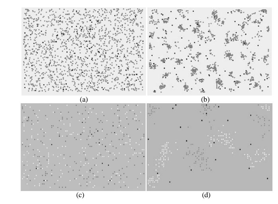
Figure 6 ACC basic model simulation, (a) RLA (black) and objects (light gray) at t = 0; (b) The objects in clusters at t = 100000; (c) RLA (black) and objects (white and light gray) in the first iteration; and (d) the current t = 570000, unloaded-RLA is black and loaded-RLA is dark gray.
A simulation of RLA using BM in a 2D-grid is shown in Figure 6(a) and Figure 6(b) for one type of object, and Figure 6(c) and Figure 6(d) for two types of objects. Experiments (a) and (b) used a parameter grid size of 290×200, number of objects = 1500, the number of RLA = 100, k1 = 0.1, k2 = 0.3 and memory m = 50, while (c) and (d) for the two types of objects (white and light gray) with 80×49 grid size, the number of white and light gray objects = 200 for each type, RLA = 20, k1 = 0.1, k2 = 0.3 and memory m = 15. Figure 7 shows ppick and pdrop for different memory lengths. The RLA memory size that was used to remember the T last steps and count the number of encountered objects, affected \(p_{pick}\) and \(p_{drop}\) values. For m=10, \(k_{pick}=0.1\) and \(k_{drop}=0.3\) it was shown \(p_{pick}\) decreased significantly and \(p_{drop}\) rose sharply. Small changes in the number of objects found by RLA (n) on the T last steps caused large changes in \(p_{pick}\) and \(p_{drop}\).
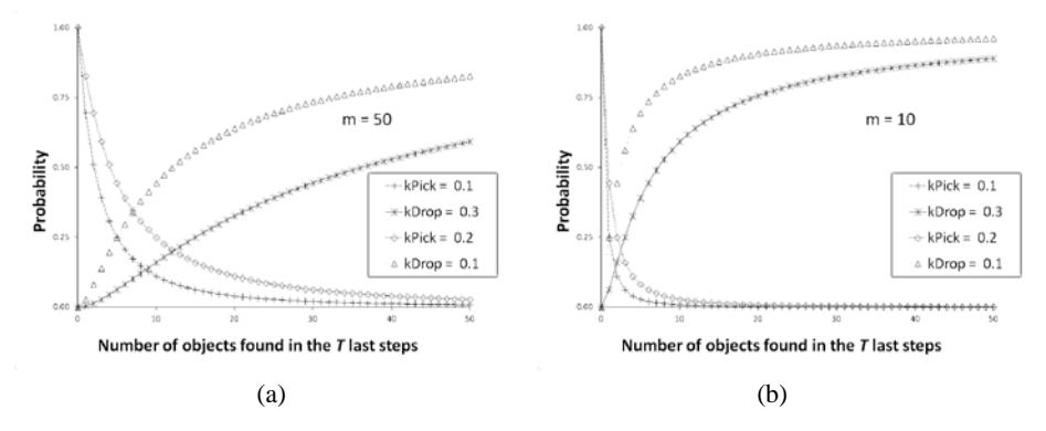
Figure 7 The number of objects found in the T last steps and their probability on different values of k with the memory size (a) m = 50 and (b) m = 10.
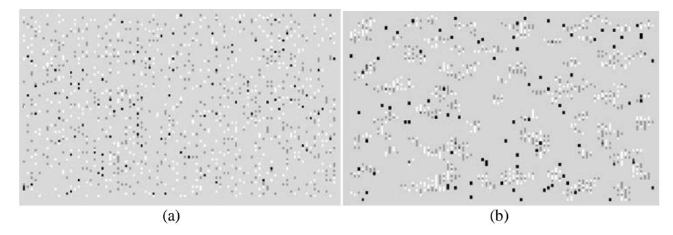
Figure 8 LF simulation with two types of objects, normal (white) and attack (light gray), (a) at t = 0 and (b) at t = 100000, unloaded-RLA (black) and loaded-RLA (dark gray).
Examples of the LF simulation results are shown in Figure 8, using a \(80\times80\) grid size, number of objects = 1000, number of RLA = 100, \(k_1\) = 0.1, \(k_2\) = 0.3 and \(\alpha\) = 50. Simulation of RLA using the LF algorithm with modification in dissimilarity using Euclidian distance measure, \(\delta(i,j)\), was replaced by using Bray-Curtis (BC) dissimilarity, \(BC_{ij} = \frac{\sum_{k=1}^{n} |x_{ik} - x_{jk}|}{\sum_{k=1}^{n} (x_{ik} + x_{jk})}\), as shown in Figure 9. The experiment was executed for two types of objects in a 80×80 grid size, number of objects = 750, number of RLA = 100, \(k_1\) = 0.1, \(k_2\) = 0.3 and \(\alpha\) = 0.7. The LF
result showed that t had decreased significantly from 100000 to 10000 when the clusters began to form. ACC was able to cluster in a distributed manner, inspired by the behavior of ant colonies while taking care of their larvae. Although ACC seems less efficient than hierarchical sorting techniques, in a distributed environment it offers advantages in terms of simplicity, flexibility and robustness. This model can be applied to two or more types of attack objects in a 2D grid space by modifying the equations δ(i,j), f(i), ppick, pdrop, and parameters used such as α, grid size, k1, k2, etc.
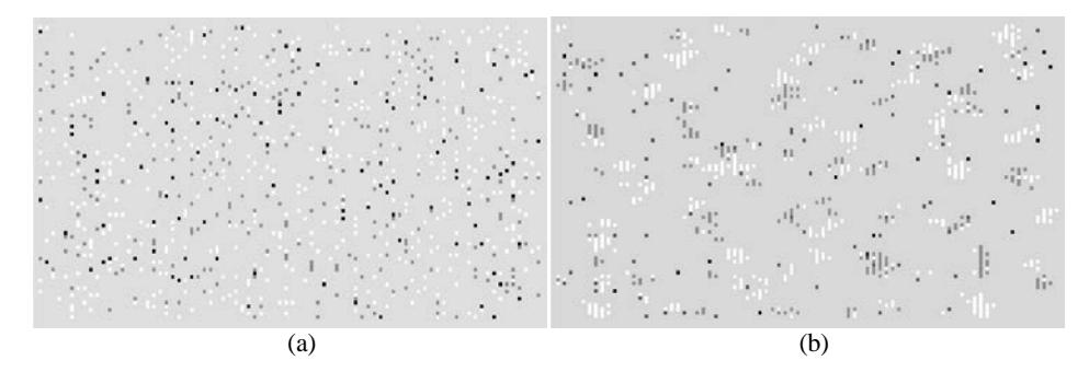
Figure 9 Simulation of modified LF δ(i,j) with BC dissimilarity, where white is normal and light gray is Satan probe attack, (a) at t = 0 and (b) at t = 10000, unloaded-RLA (black) and loaded-RLA (dark gray).
5 Conclusion
5.1 Dimensional Reduction
The use of PCA can overcome the burden of high dimensional data in the development of IDS to build a mechanism of detecting network probing activities. The initial features are transformed into new features by reducing the dimensions of the data in order to identify the characteristics of network probing activity.
Using the sign of the average value of the PCA transformation of network probing activities is useful for selecting new subsets of lower dimension. The characteristics of the relationship between PCA transformation and the initial features were identified from the values of factor loading. FAC_1 represents SYN error and REJ error when connecting to the same IP and destination port or to the same IP on different services. FAC_2 represents a SYN error when connecting to the same IP and port number in 2 seconds of time-windowing and 100 connections of connection-windowing.
FAC_4 indicates the emergence of a "not found" error and the operation as root. FAC_8 indicates the presence of a factor that created a file. FAC_9 indicates data (bytes) sent from the IP source when the connection took place. FAC_10 shows a factor of data (bytes) received during the connection. FAC_11 shows an error that occurs when the connection is logged. FAC_13 indicates a controlling file factor during connection.
Dimensional reduction of the data up to 75% of the initial features, using characteristic signs of the average value of probing activity, is perhaps able to improve the classification performance or clustering result.
5.2 ACC Algorithm
ACC as a method of attack detection is very promising. Clustering in a 2D grid space of large dimension data can be visualized and provides opportunities in controlling the process to further improve ACC performance in its application in a Distributed IDS.
Metaphorically speaking, ACC's behavior in a DIDS can be controlled and designed. It provides the ability to cluster data without guidance, to move in an unlimited 2D search space, to control the patterns of ant movement and use them to generate clusters of different types of data for normal and attack activity.
6 Future Work
Future work may include the following items:
- 1. Testing the PCA-based feature selection and extraction mechanism for the next task by using the subset formed in some classifier or clustering method that shows better performance.
- 2. Testing the performance of clustering results in a contingency table to determine the value of precision, recall, F-measure, and the ROC curve.
- 3. Designing IDS as an agent in a distributed network environment that communicates using a framework of interest-driven, cooperative agents.
- 4. Solving issues in combining a cluster model built by any IDS using an ACC algorithm in a subnet to perform the aggregated cluster model from any IDS.
- 5. Solving issues in labeling attack and normal clusters, and labeling the attack clusters according to their sub-type and not just the attack label.
- 6. Exploring some measurements in evaluating the quality of the clusters for optimizing the formed clusters with the ACC algorithm.
- 7. Further exploring the ability to accept new data to do clustering without repeating the process from the beginning.
8. Demonstrating the capability and flexibility of the system's adaptive nature to environmental changes.