
1 Introduction
Transmission lines are the most used components in electrical engineering. In many applications, transmission lines are utilized to convey energy and information from one position to another. At higher frequencies, radio frequency or microwave applications, they are exploited as network elements; they are designed as signal processing components, for example as filters. In the theory of transmission lines several characteristic quantities (R', L', C' and G') are defined. Nonuniform transmission lines, which have position varying quantities, can be used to design a matching circuit [1], a delay equalizer [2], filters [3], wave shaping [4], processing of analog signals [5], and VLSI interconnections [6].
From the theory of transmission lines, two coupled differential equations of the first order can be derived from the circuit model. These equations give the relationship between voltage and current. Eliminating one of these electric quantities leads to a differential equation of the second order. This differential equation for nonuniform cases can be solved analytically without approximation just for a few special types of NTLs: linear [7], exponential [8], power-law [9, 10], binomial [11], exponential power law [12], and hermite [13] types. For other general varying characteristic quantities, approximation methods are introduced. These methods are based on the expansion of some describing functions with unknown amplitudes, i.e. expansion of Taylor's series [14], expansion of Fourier series [15], and application of numerical computations, such as method of moment [16] and finite element method [17].
In this work we implement the same approach as described in [16]. Method of moment is a numerical approach for solving an integral equation in which we have an unknown integrand. In method of moment, the unknown function is approximated by a series of simple basis functions with unknown amplitudes. By sampling the equation in several positions, the integral equation can be converted into a system of linear equations. By inverting this matrix we can get the distribution of voltage and current along the transmission line. In this work, we observe several simple cases, such as lossless and lossy uniform transmission lines with matching and arbitrary load. These canonical cases should verify the algorithm developed in this work. The second example concerns NTLs in the form of abruptly changing transmission lines. This structure was used to design a low pass filter. A computer code based on MATLAB was developed to calculate the reflection and transmission factors of such NTLs.
2 Related Works on Nonuniform Transmission Lines
In [1] Khalaj-Amirhosseini introduced a method to synthesize microstrip NTLs for matching two arbitrary complex frequency-dependent impedances in a wideband or multi-band frequency range. In synthesizing the structure, he used a Fourier series [8]. The characteristic impedance function of the microstrip NTL was expanded by means of a truncated Fourier series. The unknown coefficients were obtained by optimizing certain frequency responses for the matching circuit. The usefulness of the proposed method was verified using wideband and dual-band matching between resistors and capacitors. It was observed that the solutions yielded a good impedance matching and as the length of the matcher was chosen larger its efficiency was increased.
In [18], formulations for reflection and transmission factors of NTLs with unequal reference impedances have been proposed. By using the ABCD matrix, the reflection and transmission factors were expressed as polynomial ratios in Z transforms. These formulations, in conjunction with techniques in digital signal
processing (autoregressive moving average process) and a reconstruction method, lead to the realization of nonuniform lines that satisfy prescribed scattering characteristics in the frequency domain. A predefined low pass filter with a step-wise transmission factor was designed and verified by measurements.
Juric-Grgic, et al. in [19] present a finite-element frequency domain model for numerical solution of the coupled nonuniform transmission line problem. Based on the finite-element method, a novel numerical procedure for solution of a system of the nonuniform multi-conductor transmission line equations in the frequency domain was presented. The results obtained by the proposed method were compared to the analytical solution.
Khalaj-Amirhosseini has proposed a method for the analysis of arbitrarily loaded lossy and dispersive single or coupled nonuniform transmission lines (NTLs) [16]. In this work, based on the available differential equations for the voltage and current, the governing integral equations for the NTLs were derived and solved using the method of moments. It was assumed that per-unit-length matrices are known along the whole length or at some positions of the coupled NTLs. The method of moment in this work used rectangular pulse function expansion with point matching. A coupled transmission line pair was observed and the calculated voltage distribution along the excited line and along the unexcited line was compared with the exact results.
Lu [7] has given the analytical solution of an ideal linear varied NTL (LNTL), including the exact linear two-port ABCD matrix of the LNTL. Based on this result, he cascaded the LNTL sections to approximate an arbitrary characteristic impedance profile and presented a technique for analyzing an arbitrary NTL. The technique is better than the conventional technique in terms of computational accuracy and intensity since it uses a piecewise linear characteristic impedance profile in place of the stepped profile used by the conventional technique.
In other publications [20,21] NTLs were used for designing dual-band and multiband power dividers. In this paper, the NTLs were subdivided into small sections, described by ABCD matrices and the ABCD matrix of the whole structure could be obtained just by multiplication of all sub ABCD matrices. For modeling the normalized characteristic impedance, the truncated Fourier series expansion was used. The optimum values of the Fourier coefficients could be obtained through minimization of a certain error function, which quantifies the difference between the obtained ABCD matrix and desired ones. The Wilkinson power dividers designed here can be set to work in dual band or multiband, depending on the ABCD matrix target.
3 Wave Equation of Nonuniform Transmission Lines and Its Solution
In two-conductor transmission lines the voltage and current can be defined uniquely. If the cross-section of the transmission lines is small enough compared to the wavelength, the voltage and current are related to each other by the following equations
\[\frac{dV(z)}{dz} = -Z'(z)I(z) \tag{1}\]
\[\frac{dI(z)}{dz} = -Y'(z)V(z) \tag{2}\] with arbitrarily position-varying parameters \(Z'(z) = R'(z) + j\omega L'(z)\) and \(Y'(z) = G'(z) + j\omega C'(z)\), and z is the direction of the propagation. R', L', G' and C' are the primary parameters of the transmission lines.
By eliminating the current, Eqs. (1) and (2) lead to a nonhomogeneous differential equation of the second order,
\[\frac{d^{2}V(z)}{dz^{2}} - f(z)\frac{dV(z)}{dz} - \gamma^{2}(z)V(z) = 0\] (3)
with f(z) = (dZ'/dz) Z' and \(\gamma^2 = Z'Y'\).
The solution of Eq. (3) is not simple and is available analytically only for some special functions of Z' and Y'. To give a solution for the problem, this paper takes the integrals of Eqs. (1) and (2) with respect to z leading to
\[V(z) = -\int_0^z Z'(z')I(z')dz' + C_1\] (4)
\[I(z) = -\int_0^z Y'(z')V(z')dz' + C_2\] (5)
The integration constants, \(C_1\) and \(C_2\), can be derived from the boundary conditions given in Figure 1, which are,
\[C_1 = \frac{Z_L}{Z_I + Z_I} V_S + \frac{Z_I}{Z_I + Z_I} \int_0^d [Z'(z')I(z') - Z_L Y'(z')V(z')] dz'\]
\[C_2 = \frac{1}{Z_i + Z_L} V_S - \frac{1}{Z_i + Z_L} \int_0^d [Z'(z')I(z') - Z_L Y'(z')V(z')] dz'\]
If we set as value for z = 0 in Eq. (4), the integral vanishes and the equation becomes \(V(z = 0) = C_1\). Physically this means that \(C_1\) is the voltage measured at position z = 0 and analogous, if Eq. (5) is used for z = 0, it leads to \(I(z = 0) = C_2\), so \(C_2\) is the current at position z = 0.
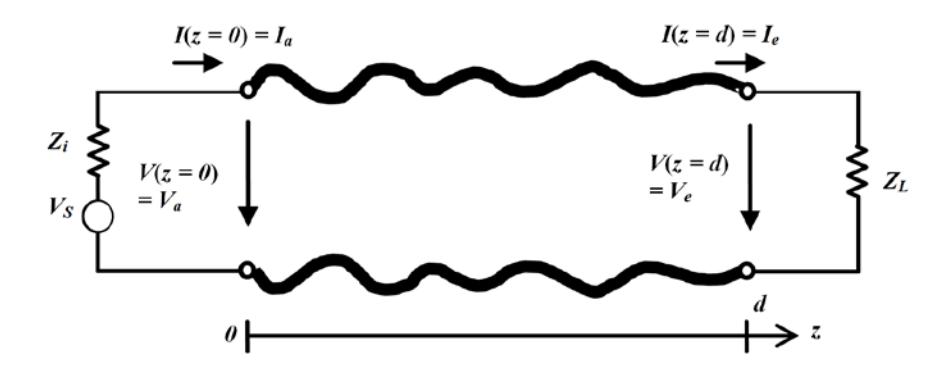
Figure 1 Nonuniform transmission line of length d with source VS and internal impedance Zi and load ZL.
Eqs. (4) and (5) are integrals of unknown current and voltage along the transmission line. These equations are coupled to each other, so that solving the problem must include the equations simultaneously. In order to approximate the unknown voltage and current distribution, it is worthy to express the voltage and current as a linear combination of the so-called basis functions with unknown amplitudes,
\[V(z) = \sum_{n=1}^{N} V_n f_n(z)\] (6)
\[I(z) = \sum_{n=1}^{N} I_n f_n(z)\] (7)
fn are simple known basis functions, Vn and In are the unknown constants, and N is the number of approximating functions. In this case, we have 2 × N unknowns.
Inserting Eqs. (6) and (7) into Eqs. (4) and (5) we get,
\[\sum_{n=1}^{N} V_{n} \left[ f_{n} + \frac{Z_{i}Z_{L}}{Z_{i} + Z_{L}} \int_{0}^{d} Y' f_{n} dz' \right] + \sum_{n=1}^{N} I_{n} \left[ \int_{0}^{z} Z' f_{n} dz' - \frac{Z_{i}}{Z_{i} + Z_{L}} \int_{0}^{d} Z' f_{n} dz' \right]\] \[= \frac{Z_{L}}{Z_{i} + Z_{L}} V_{S}\] and,
\[\sum_{n=1}^{N} V_{n} \left[ \int_{0}^{z} Y' f_{n} dz' - \frac{Z_{L}}{Z_{i} + Z_{L}} \int_{0}^{d} Y' f_{n} dz' \right] + \sum_{n=1}^{N} I_{n} \left[ f_{n} + \frac{1}{Z_{i} + Z_{L}} \int_{0}^{d} Z' f_{n} dz' \right] = \frac{V_{S}}{Z_{i} + Z_{L}} \int_{0}^{d} Z' f_{n} dz' dz' dz' dz' dz' dz' dz'\]
These equations can be given in a compact matrix form as follows,
\[\begin{pmatrix} A & B \\ C & D \end{pmatrix} \begin{pmatrix} V \\ I \end{pmatrix} = \frac{V_S}{Z_I + Z_L} \begin{pmatrix} Z_L \\ 1 \end{pmatrix}\] (8)
where \(V = \begin{bmatrix} V_1 & V_2 & \dots & V_N \end{bmatrix}^T\) and \(I = \begin{bmatrix} I_1 & I_2 & \dots & I_N \end{bmatrix}^T\) are the unknown vectors and four known \(1 \times N\) matrices A, B, C and D, whose elements are,
\[A_n(z) = f_n(z) + \frac{Z_i Z_L}{Z_i + Z_L} \int_0^d Y'(z') f_n(z') dz'\] (9)
\[B_n(z) = \int_0^z Z'(z') f_n(z') dz' - \frac{z_i}{z_i + z_L} \int_0^d Z'(z') f_n(z') dz'\] (10)
\[C_n(z) = \int_0^z Y'(z') f_n(z') dz' - \frac{Z_L}{Z_I + Z_L} \int_0^d Y'(z') f_n(z') dz'\] (11)
\[D_n(z) = f_n(z) + \frac{1}{Z_i + Z_L} \int_0^d Z'(z') f_n(z') dz'\] (12)
Evaluation of the integrals in Eqs. (9) to (12) can be performed effectively in the computer by dividing the transmission line into small segments, i.e. the transmission line is discretized into N segments. In case of uniform discretization, the segment length \(\Delta z\) is equal to d/N. The complexity of the integral calculation can be substantially reduced if we use as the basis function a constant function in each segment, i.e.,
\[f_n = \begin{cases} 1 & \text{for } (n-1)\Delta z \le z \le n\Delta z \\ 0 & \text{otherwise} \end{cases}\] (13)
The choice of the basis function in Eq. (13) leads to simplification of the integral along 0 to d and along 0 to z. For example, the integral in Eq. (9) delivers results different than zero just along the small segment \((n-1)\Delta z \le z \le n\Delta z\). Furthermore, if the transmission line is discretized fine enough, i.e. N is large, \(\Delta z\) becomes small enough, then we can approximate the integration just by a simple multiplication between the segment length \(\Delta z\) and the mean value of Z or Y, or by just taking the value of Z or Y at the midpoint of the segment \(z_n\). These results are valid for all \(0 \le z \le d\). However, in order to solve the problem with \(2 \times N\) unknowns uniquely, we must choose N special positions to get in total \(2 \times N\) equations. These special positions are called testing points. A simple procedure is to use the collocation method. In this method, we choose the middle point of each segment \(z_m\), so that the approximate values of \(A_n\), \(B_n\), \(C_n\) and \(D_n\) at the position \(z_m\) become,
\[A_n(z_m) = \delta_{mn} + \frac{z_i z_L}{z_i + z_L} Y'(z_n) \Delta z \tag{14}\]
\[B_n(z_m) = Z'(z_n)U_{mn}\Delta z - \frac{z_i}{z_i + z_i}Z'(z_n)\Delta z\] (15)
\[C_n(z_m) = Y'(z_n)U_{mn}\Delta z - \frac{z_L}{z_i + z_L}Y'(z_n)\Delta z\] (16)
\[D_n(z_m) = \delta_{mn} + \frac{1}{Z_i + Z_L} Z'(z_n) \Delta z \tag{17}\]
δmn is the Kronecker function and,
\[U_{mn} = \begin{cases} 1 & \text{for } m > n \\ 1/2 & \text{for } m = n \\ 0 & \text{for } m < n \end{cases}\]
Which means that if the observation position is on the right side of the integration boundary (m > n), we get the full integration. If the observation position is located exactly at the middle of the integration range, it yields half of the result. And if the observation position is on the left side of the integration range (m < n), the integration gives the value zero.
The collocation method is a type of method of moment, whose basis function uses pulse function and as test function a delta function is used.
From the information on the voltage distribution along the structure, we can extract the standing wave along the connecting line on the source side, from which we can calculate the voltage standing wave ratio by,
\[VSWR = \frac{V_{max}}{V_{min}} \tag{18}\]
Vmax and Vmin are the maximal and minimal value of the voltage along that connecting line, respectively. From these values, we can calculate the reflection factor S11 and incident as well as reflected voltages.
From the voltage distribution along the connecting line on the load side, we can also obtain the transmitted voltage. By dividing this value by the incident voltage, we can calculate the transmission factor S21.
4 Simulation Results
In this work, firstly we observed uniform transmission lines with matching and arbitrary loadings. As additional parameter we used lossless and lossy transmission lines. We designed and analyzed two low pass filters as practical implementation of NTLs.
4.1 Voltage Distribution along Uniform Transmission Lines
A 60 cm length uniform transmission line was observed. The transmission line had a constant capacitance per unit length C' = 66.7 pF/m and inductance per unit length L' = 0.167 μH/m. By ignoring any losses, a wave impedance of about Zo = 50 Ω for the lossless case was obtained independent of frequency. The transmission line was connected with a load of ZL = 50 Ω and excited by a voltage source VS = 1 V with a frequency of f = 1 GHz and an internal impedance of Zi = 50 Ω. In this example, we set G' = 0 and make a variation on the resistance per unit length R'.
Figure 2 shows the voltage distribution along the transmission line for different losses. For the lossless case, we see a constant curve, which means there is no standing wave. The value of voltage standing wave ratio (VSWR) is 1, which means we do not have any reflected waves. For lossy cases (R' > 0), the propagating waves experience attenuation along the transmission line. Figure 2 illustrates that the larger the resistance per unit length, the smaller the amplitude of the voltage apart from the source. Interestingly, in case of higher losses, for this 'matching' condition, we observe a standing wave in the form of small ripples. Such ripples must originate from superposition between incident and reflected waves. In this case, reflection indeed happens. With losses (R'≠0), the value of the wave impedance is no longer 50 Ω. For example, with R' = 250 Ω/m, we get a complex wave impedance of (50.3864 - j5.9196) Ω. This yields together with the load ZL = 50 Ω a reflection factor of |r| = 0.059, or a VSWR of 1.1254.
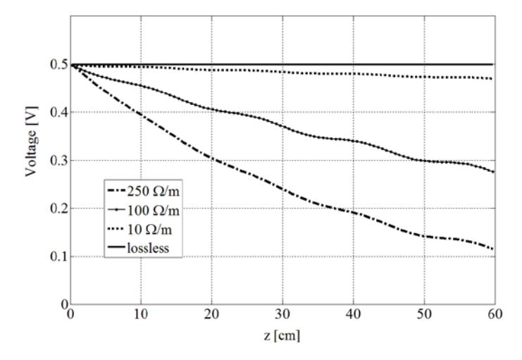
Figure 2 Voltage distribution along transmission line with matching loading in dependence on resistance per unit length R'.
In order to study the effect of losses on the standing wave, we now replaced the load by an impedance ZL = 20 Ω. Connecting this load to a transmission line with a wave impedance of 50 Ω leads to a reflection factor r = −0.4286 or VSWR= 2.5. For the lossless case in Figure 3, the standing wave pattern does not change along the transmission line. The maximal voltage of Vmax = 0.7143 V and the minimal voltage of Vmin = 0.2857 V can be read, whose ratio is exactly equal to the value of VSWR given above. At the load position, we have a minimum, because the load impedance is smaller than the wave impedance of the transmission line, as verified by the theory.
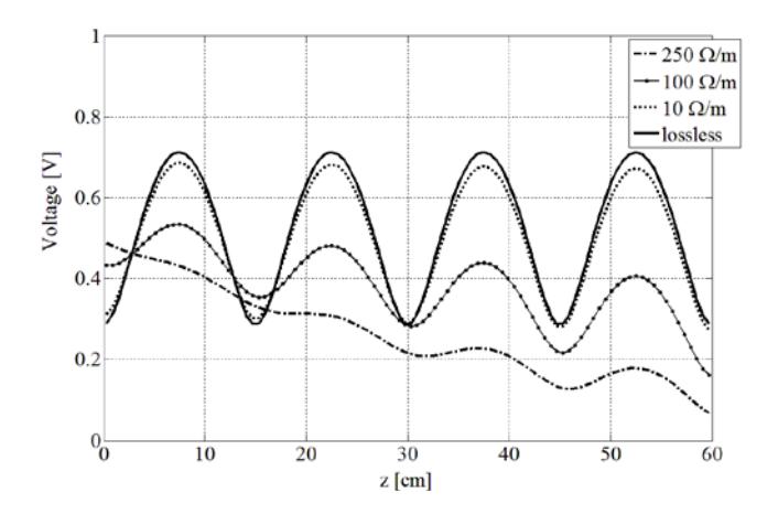
Figure 3 Voltage distribution along transmission line with ZL = 20 Ω in dependence on resistance per unit length R'.
By including losses in the calculation, the standing wave pattern changes along the structure substantially. We observe smaller VSWR at positions near to the source than near to the load. From the theory of lossy transmission lines, we have learnt that the incident wave from the source to the load is attenuated and after being reflected by the load back to the source, the reflected wave is attenuated again. This makes the contribution of the reflected wave to the standing wave pattern near the source small as compared to the lossless case. Hence, for very lossy cases, near to the source the value of Vmax is practically equal to the value of Vmin and any reflections, even total reflection, can be neglected.
4.2 Chebychev's Low Pass Filters based on Stepwise Nonuniform Transmission Lines
Microwave filters play a significant role in modern communication systems [22]. Designing microwave filters is an interesting combination between creativity and possibility. One of the most basic design procedures is approximating the ideal characteristics of low pass filters with Chebychev's functions. Approximation of filtering characteristics with Chebychev's functions relies on the number of components used, i.e. the order of the filter N and on the ripple allowed in the pass band. Figure 4 shows the generic form of a low pass filter designed by this approximation.
Figure 4 Generic form of low pass filter approximated by polynomial functions.
The value of each component in Figure 4 can be obtained in many textbooks, which is given in tabularized form in Table 1. The data given in this table is the standard information valid for any reference impedance and frequency. For special load or internal impedance, for example 50 Ω and a special reference frequency, for example ωc = 2π . 109 rad/s, we must multiply the inductance value by the impedance and divide by the radial frequency ωc, and divide the capacitance value by the impedance and again by the radial frequency.
Table 1 Element Values for Chebychev Low Pass Prototype for Normed Impedance Zi = 1, Frequency Ω = 1 and Ripple 0.3 dB for Filter Order up to 5.
| N | g1 | g2 | g3 | g4 | g5 | g6 |
|---|---|---|---|---|---|---|
| 1 | 0.5349 | 1.0000 | ||||
| 2 | 1.1805 | 0.6957 | 1.6967 | |||
| 3 | 1.3713 | 1.1378 | 1.3713 | 1.0000 | ||
| 4 | 1.4457 | 1.2537 | 2.1272 | 0.8521 | 1.6967 | |
| 5 | 1.4817 | 1.2992 | 2.3095 | 1.2992 | 1.4817 | 1.0000 |
In this study, a low pass filter with order N = 3 and ripple 0.3 dB was designed with fc = 1 GHz and reference impedance of Z0 = 50 Ω. The element values given in Table 1 become the following values of inductances and capacitances,
\[g_1 = 1.3713\] \(\rightarrow\) \(L_1 = 10.91 \text{ nH}\)
\(g_2 = 1.1378\) \(\rightarrow\) \(C_2 = 3.6219 \text{ pC}\)
\[g_3 = 1.3713\] \(\rightarrow\) \(L_3 = 10.91 \text{ nH}\)
In microstrip technology, inductances can be modeled by a high impedance microstrip line (Z0L > Z0) and capacitances by a low impedance microstrip line (Z0C < Z0). The choice of the impedance values Z0L and Z0C are rather arbitrary, however, restrictions are that the value of Z0L may not be too high, which could yield a very thin strip line that is difficult to be fabricated, and that the value of Z0C may not be too low, which leads to a wide strip line that can cause a transversal wave propagation in this microstrip segment. Here, a TMM10 substrate [23] with a relative permittivity of 9.2, a tangent loss of 0.0022 and a thickness of 2.54 mm was used. Table 2 gives an overview of the relationship between the set impedance values and the widths of the microstrip lines, which were designed by the standard design equation given as an example in [24].
| Z0 [Ω] | W [mm] | εr,eff | λg at fo= 1 GHz [mm] |
|---|---|---|---|
| 50 | 2.62 | 6.31 | 119.345 |
| 86.7 | 0.64 | 5.79 | 124.627 |
| 30 | 6.34 | 6.94 | 113.806 |
Table 2 Design Data for Low Pass Filter.
In order to get each value of inductance and capacitance given above, the microstrip lines must have certain lengths, which fulfill the following equations [24],
\[2\pi f_o L = Z_{0L} \sin\left(\frac{2\pi l_L}{\lambda_{gL}}\right) + Z_{0C} \tan\left(\frac{\pi l_C}{\lambda_{gC}}\right)\] (19)
\[2\pi f_o C = \frac{1}{Z_{oC}} \sin\left(\frac{2\pi l_C}{\lambda_{gC}}\right) + \frac{2}{Z_{oL}} \tan\left(\frac{\pi l_L}{\lambda_{gL}}\right)\] (20)
Applying these coupled equations and the data given in Table 1 with an iterative method, we get the values lL = 15.00 mm and lC = 10.63 mm. Figure 5 shows a microstrip circuit for this low pass filter.
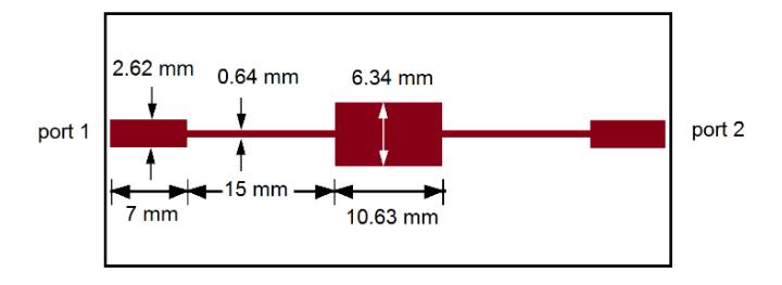
Figure 5 Low pass filter of order N = 3 with two 50 Ω feeding lines.
On the source and load sides, two connecting transmission lines with a wave impedance of 50 Ω were connected and we connected an internal impedance ZS = 50 Ω and a load impedance ZL = 50 Ω, so that both sides were in matching condition. In order to extract the voltage distribution along the connecting lines, we used 150 mm and 10 mm long lines on the source and load sides, respectively. Our target here was to analyze the low pass filter structure in the frequency range between 100 MHz and 1.5 GHz. We calculated the reflection factor (S11) and transmission factor (S21) of the filter. The reflection emerges not due to the load, but rather due to the nonuniform structure of the transmission line used (causing abrupt changes of the impedance). It could be verified later if we had a constant voltage distribution along the connecting line on the load side. It was indeed, because there is just a wave propagating to the load. However, along the connecting line on the source side, we expected a standing wave pattern, having a maximum and minimum voltage. From this pattern we could calculate the VSWR and then the reflection factor.
Figure 6 shows the voltage distribution along the transmission line at a frequency of 1.5 GHz. The curve on the load side (190 mm < z < 200 mm) was constant; this is the voltage wave towards the load with value Vt = 0.2822 V. On the source side (z < 150 mm), we had a standing wave pattern with Vmax = 0.9096 V and Vmin = 0.0904 V, which yielded a VSWR of 10.0619 or a reflection factor of 0.8192 (= −1.732 dB). On the source side, we could calculate the voltage wave propagating to the input side of the filter with Vinc = 0.5(Vmax+Vmin) = 0.5 V, so that the transmission factor could be calculated to t = 0.2822/0.5 = 0.5643 (= −4.970 dB).
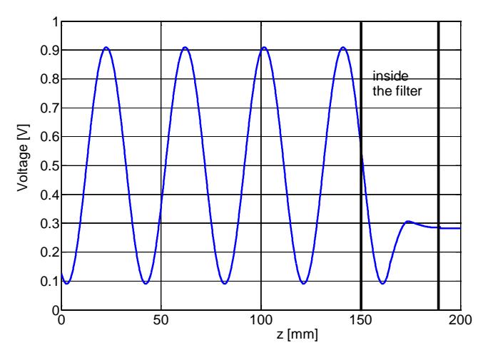
Figure 6 Voltage distribution inside the low pass filter and along its connecting lines at frequency 1.5 GHz.
In Figure 6, the maximal voltages on the source side are about 40 mm apart from each other, which is exactly half of the guided wavelength from the theory of transmission lines.
At lower frequencies, i.e. 600 MHz, we expected the maxima to be separated by longer distances. With the same procedure used as for Table 2, we got a guide wavelength of about 199.66 mm for 600 MHz. The connecting line with a length of 150 mm was still enough for observing the standing wave as shown in Figure 7. The maximal voltage of 0.5460 V and the minimal voltage of 0.4540 V delivered a VSWR of 1.2026 or a reflection factor of 0.092 (= −20.725 dB). With the voltage at the load side Vt = 0.4951 V and the incident voltage on the source again Vinc = 0.5(Vmax + Vmin) = 0.5 V, so that the transmission factor could be calculated as t = 0.4951/0.5 = 0.9901 (= −0.0863 dB).
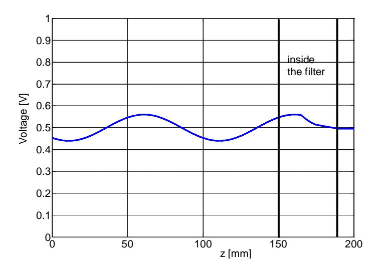
Figure 7 Voltage distribution inside the low pass filter and along its connecting lines at frequency 600 MHz.
By varying the frequency from 100 MHz to 1.5 GHz, we could calculate the reflection and transmission factors over this frequency range. The result is depicted in Figure 8. For comparison purposes, a prototype of the low pass filter was fabricated and measured. We observed a deviation of about 0.7 dB in the transmission factor and some oscillation in the measured reflection factor, which could come from the cable of the network analyzer. We found the minimum of the reflection factor at about 725 MHz. In general, we saw a very good similarity between both results.
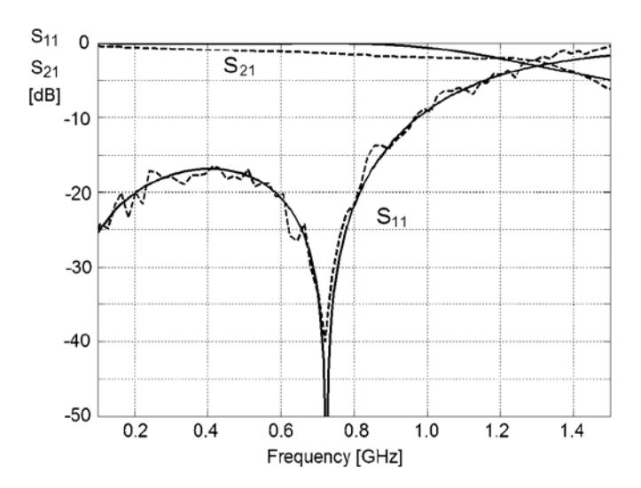
Figure 8 Scattering parameters of low pass filter N = 3. Solid lines: this work. Dashed lines: measured by network analyzer ZVL13.
In order to enhance the selectivity of the filter, a second filter with N = 5 was considered. With the same impedance and frequency reference as the previous filter and the element values given in Table 1, we got the following values of inductance and capacitance,
\[g_1 = 1.4817\] \(\Rightarrow\) \(L_1 = 11.79 \text{ nH}\)
\(g_2 = 1.2992\) \(\Rightarrow\) \(C_2 = 4.136 \text{ pC}\)
\(g_3 = 2.3095\) \(\Rightarrow\) \(L_3 = 18.38 \text{ nH}\)
\(g_4 = 1.2992\) \(\Rightarrow\) \(C_4 = 4.136 \text{ pC}\)
\(g_5 = 1.4817\) \(\Rightarrow\) \(L_5 = 11.79 \text{ nH}\)
Figure 9 shows a microstrip circuit for this low pass filter of order N = 5. The substrate used was the same as before. The dimensions were calculated again by solving the nonlinear Eqs. (19) and (20) iteratively.
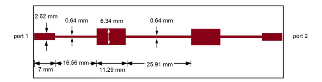
Figure 9 Low pass filter of order N = 5 with two 50 Ω feeding lines.
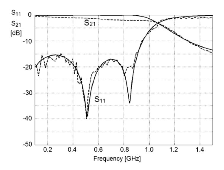
Figure 10 Scattering parameters of low pass filter N = 5. Solid lines: this work. Dashed lines: measured by network analyzer ZVL13.
The characteristic filtering is shown in Figure 10. This filter had a sharper curve between the pass and stop regions compared to the low pass filter with N = 3. The comparison of the results found here and the measurements also showed coincidences. The minimums of the reflection factor were observed at frequencies 510 MHz and 845 MHz.
5 Conclusion
The implementation of method of moment as solution for integral equations in nonuniform transmission lines yields very good results. Some canonical problems, such as matching and unmatched load connected to uniform transmission lines with and without losses, verified the computer simulation. The numerical results coincided with those yielded by the theoretical approach. Finally, abruptly changing nonuniform transmission lines, which presents itself as Chebychev's low pass filters, was considered. The results were compared with measurements. For each filter design we observed the minimum of the reflection factor and a sharper transition between the pass and stop regions. In general, the comparison showed very good coincidences.
Acknowledgements
This research is supported by the Directorate of Higher Education, Republic of Indonesia under the scheme of Decentralization Research Grant 2014. The authors would like to express their thanks for the financial support.