
1 Introduction
An image compression algorithm generally involves a transformation to compact most of the pixels' energy into a few numbers of decorrelated coefficients that are easier to code. The transformed coefficients are then quantized and encoded to produce the compressed bitstream. The most widely used transforms for image compression applications are the discrete cosine transform (DCT) and the discrete wavelet transform (DWT). DCT has low complexity and excellent energy compaction. DCT is non-local and hence it is not practical to apply it to the whole image. Instead, DCT is implemented as block-based transform by which the image is normally divided into a number of non-overlapping blocks of (8×8) or (16×16) pixels and the separable twodimensional discrete cosine transform (2D-DCT) is applied to these blocks
Received February 1st, 2015, 1st Revision August 23rd, 2015, 2nd Revision November 2nd 2015, Accepted for publication November 6th, 2015.
Copyright © 2015 Published by ITB Journal Publisher, ISSN: 2337-5787, DOI: 10.5614/itbj.ict.res.appl.2015.9.3.2
individually. Unfortunately, the block-based DCT suffers from annoying blocking artifacts near the edges of the blocks. These artifacts lead to discontinuities at the block boundaries, especially at low bit rates. Nevertheless, DCT has been used for image and video compression and conferencing standards such as JPEG, MPEG, and H.263 due to its low complexity and excellent compaction features [1,2].
On the other hand, 2D-DWT, in addition to its good energy compaction, has additional features such as its space-frequency localization property and multiresolution capabilities. The localization property permits DWT to be applied to the entire image, which eliminates the blocking artifacts and facilitates rate scalability. The multi-resolution capabilities facilitate resolution scalability, which permits reconstructing the image in several sizes. Unfortunately, the computational time of DWT is longer than that of DCT, as 2D-DCT requires only 54 multiplications to transform a block of 64 pixels, while 2D-DWT requires at least one multiplication per pixel [3]. In addition, 2D-DWT suffers from a blurring and ringing effect near edge regions in the image [4].
2D-DWT is usually applied several times to the image, producing what is called pyramidal hierarchical decomposition. For example, dyadic 2D-DWT decomposition first decomposes the image into four subbands, labeled LL1, LH1, HL1, and HH1. The second stage decomposes the LL1 subband into four subbands, labeled LL2, HL2, LH2, and HH2. This recursive decomposition for the LL subband can be performed K times resulting in 3K+1 subbands. Figure 1 depicts dyadic DWT decomposition for three stages (K = 3). It can be shown that the best DWT efficiency can be obtained with K = 5 [5].
| HH1 | HH1 | HH1 | HH1 | HH1 | HH1 | ||||
|---|---|---|---|---|---|---|---|---|---|
| LH2 | HH2 | LH2 | HH2 | HL1 | |||||
| LL1 | HL1 | LL2 | HL2 | HL1 | LL3 LH3 | HL3 HH3 | HL2 | ||
Figure 1 Three stages of dyadic 2D-DWT decomposition.
A rate scalable image compression system generates a compressed bitstream that can be truncated at any point while maintaining the best possible image quality for the selected bit rate. This property is a very interesting feature for the modern heterogeneous networks as users may have different resource capabilities in terms of processing speed, available memory and power. Accordingly, each user can request an image quality that fits his needs. In a rate scalable image compression system, the image is compressed only once at the maximum bit rate. The resulting bitstream is then stored on a server. Different users with different bit rate requirements send their requests to the server. The server then provides each user with a properly scaled bitstream that fit the user's request by simply truncating the bitstream at the target bit rate [6]. The most popular wavelet-based rate scalable image compression algorithms are the set partitioning in hierarchical trees (SPIHT) algorithm [7] and the set partitioning embedded block (SPECK) algorithm [8]. These coding schemes are very efficient and use a low complexity set partitioning technique. In this paper, we propose a new algorithm, called the ultrafast and efficient rate scalable (UFERS) algorithm. This algorithm makes use of 2D-DCT instead of 2D-DWT to work with the wavelet-based set partitioning technique in order to reduce the complexity of the overall system.
2 Literature Survey
Several algorithms have been presented in the literature that use DCT with coding techniques that were initially designed to work with DWT in order to reduce their complexity.
Yen, et al. [4] presented an algorithm that has about the same complexity as JPEG using a modified SPIHT. It considers each (8×8) DCT block consisting of 10 subbands arranged in 3 dyadic decomposition levels according to the importance of the coefficients in the DCT block. Then, the DCT coefficients that belong to the same subband from every DCT block are grouped together. The rearranged image is then encoded using the modified SPIHT. The SPIHT algorithm [7] exploits the self-similarities that exist between the wavelet coefficients of the subbands across the decomposition levels. It is worth noting that this self-similarity feature is a special attribute devoted to the dyadic 2D-DWT. Thus, the self-similarities are expected to be weak for DCT images. As such, the efficiency of the DCT-based SPIHT is expected to be moderate. However, it is claimed that the modified SPIHT increases efficiency using two additional steps, called the combination and dictator, to eliminate the correlation between the same-level subbands for encoding the DCT-based image. In addition, it makes use of an enhancement filter in order to improve the image quality at low bit rates. Evidently, these steps increase the complexity of the algorithm.
Song, et al. [9] presented a DCT-based rate scalable algorithm. It also uses the aforementioned DCT grouping method. In the coding stage, the magnitudes of the DCT coefficients are estimated by the linear sum of four coefficients at the same location in the neighboring DCT blocks, while the coefficients with larger estimates are given higher priority in encoding. This priority information is also used as context for the binary arithmetic coder that performs the actual coding. The proposed method is supposed to find more significant coefficients earlier than the conventional methods, thereby providing a higher coding gain. The algorithm has excellent performance but at the expense of highly increased complexity since the complexity of the arithmetic coder is about 4 times higher than the Huffman coder used in JPEG [10]. In addition, assigning priority to coefficients requires a sorting mechanism, which is not desirable due to its high complexity [11].
Tu, et al. [12] have presented the embedded-context-based entropy coding of block transform coefficients (E-CEB) algorithm. The algorithm adopts a different reordering method for the DCT coefficients as it combines each DCT coefficient located at the same position from every DCT block on the same subband. This is equivalent to the wavelet packet decomposition structure [2]. Unfortunately, E-CEB has about the same complexity as [9] because it also makes use of a binary arithmetic coder with context modeling.
Panggabean, et al. [13] have proposed a DCT-based algorithm that is suitable for real-time tele-immersive collaboration applications. The coder consists of three major steps: block ranking, DCT, and entropy coding using variablelength encoding and run-length encoding. The coder is very fast, rate scalable, and fully parallelized. Unfortunately, it has a lower performance than the original JPEG, which limits its practical use.
The proposed UFERS algorithm rearranges the DCT coefficients, using the same method as [4] and [9], but it employs a modified version of the SPECK algorithm in the coding stage. The motivation of using SPECK is that in addition to its good rate-distortion performance and low complexity, it exploits the correlation between the wavelet coefficients that exist within the subbands. That is, it doesn't depend on the self-similarities that exist between the wavelet coefficients across subbands. Therefore the performance of the DCT-based SPECK is expected to be better than the DCT-SPIHT from [4]. Unfortunately, SPECK has higher memory requirements and management complexity than SPIHT due to using an array of linked lists to store the sets according to their sizes. The modified SPECK presented in this paper replaces this array by two lists only, similar to those used by SPIHT.
The remainder of the paper is organized as follows. Section 3 describes the SPECK algorithm. Section 4 presents the proposed UFERS algorithm. Section 5 gives the experimental performance results of UFERS in conjunction with a comparison with several previous rate scalable algorithms. Finally, Section 6 concludes the paper.
3 The SPECK Algorithm
The SPECK algorithm [8] transforms the image to the wavelet domain using the dyadic 2D-DWT. Every wavelet coefficient is initially quantized by rounding it to the nearest integer and represented by a sign-magnitude format using B bits (e.g. 16 bits), where the first bit is the sign bit (e.g. 0 for a positive coefficient and 1 for a negative coefficient) and the other B-1 bits are the magnitude bits. The quantized DWT image (W) is then bit-plane coded, whereby the magnitude bits of the DWT coefficients are coded from most significant bit (MSB) to least significant bit (LSB). That is, the image is coded bit-plane by bit-plane rather than coefficient by coefficient. To this end, multiple coding passes through W are made. Each coding pass corresponds to a bit-plane level. The maximum bitplane nmax depends on the maximum value of the DWT coefficients in W and is given by:
\[n_{max} = \left[ log_2 max_{\forall (i,j) \in W}(|c_{ij}|) \right]\] (1)
where x is the largest integer ≤ x and cij is a quantized DWT coefficient at location (i, j) in W. nmax should be signaled to the decoder in order to start decoding at bit-plane nmax. For the following description, the term pixel is used to designate a quantized DWT coefficient.
At any bit-plane, n, nmax≥ n ≥ 0, a pixel cij is considered significant (SIG) with respect to n if 2 ≤ � � < 2+1. Otherwise cij is insignificant (ISIG). Similarly, a set of pixels T is considered SIG with respect to n if it contains at least one SIG pixel. Otherwise T is ISIG. Once a pixel is found to be SIG, it is coded by sending a '1' and its sign bit directly to the bitstream. A pixel that is still ISIG is coded by sending '0' to the bitstream. As mentioned earlier, SPECK employs the set partitioning technique to partition the SIG sets while keeping the ISIG sets. In this way a large area of ISIG pixels is coded by one bit. The same process is repeated for the new partitioned SIG sets until all pixels are encoded. The SPECK algorithm makes use of quad-tree decomposition to split off the SIG sets at the midpoint along each side into four subsets, collectively denoted as O(T), each having one-fourth the size of the parent set T, as shown in Figure 2.
Figure 2 Quad-tree partitioning of a SIG set (T) into 4 subsets O(T).
SPECK makes use of three linked lists to keep track of the pixels and sets that need to be tested and coded, called respectively: list of insignificant pixels (LIP), list of significant pixels (LSP), and list of insignificant sets (LIS). LIP stores the (i, j) coordinates of the ISIG pixels, LSP stores the (i, j) coordinates of the SIG pixels, and LIS stores the (i, j) coordinates of the root of the ISIG sets. The root of a set is represented by its top-left pixel. To simplify description, when we say a pixel is added to (or removed from) LIP or LSP, this means that the pixel's (i, j) coordinates are added (or removed). Similarly, when we say a set is added to (or removed from) LIS, this means that the root's (i, j) coordinates of the set are added (or removed).
SPECK starts coding by computing the maximum bit-plane, nmax. LIS is initialized by the 3K+1 image subbands ordered from the lowest frequency subband (LLK) to the highest (HH1); LIP and LSP are initialized empty. Each bit-plane coding pass starts with significance testing and coding the (i, j) entries of LIP, LIS, and LSP respectively against the current bit-plane (n). Each pixel in LIP is tested and coded accordingly and if it is found to be SIG, it is removed from LIP and added to the end of LSP to be refined in the next coding passes; otherwise it is kept in LIP to be tested in the next coding passes. Then, each set T in LIS is tested. If T is still ISIG, a '0' is sent to the bitstream, i.e. the entire set is coded by one bit. On the other hand, if T is found to be SIG, a '1' is sent to the bitstream, T is removed from LIS, and it is quad-tree partitioned into four subsets. Each one of these four subsets is in turn treated as a type T set and processed in the same way as the parent set. Any subset that is found ISIG during this partitioning process is added to LIS in order to be tested at the next lower bit-planes coding passes later on.
This recursive partition of the new SIG sets continues until the pixel level is reached (i.e. the set size is 2×2 pixels). At this stage, if the set is ISIG, a '0' is sent to the bitstream and if it is SIG, a '1' is sent to the bitstream and each one of its four pixels is tested and coded accordingly and if a pixel is found to be SIG, it is added to LSP in order to be refined in the next bit-planes; otherwise, if it is still ISIG, it is added to LIP in order to be tested in the next bit-planes. Finally, each pixel in LSP – except for those that were just added during the current pass – is refined to an additional bit of precision by sending its nth MSB to the bitstream. Finally, the bit-plane is then decremented by one to start a new coding pass. This cycle continues until all the bits of all pixels are encoded or until the target bit rate is reached.
It should be noted that at the end of the first coding pass (and the other passes), LIS may contain sets of varying sizes due to the adopted recursive quad-tree partitioning process. It is well known that the probability of finding SIG pixels is inversely proportional to set size. Therefore, LIS is not traversed sequentially for processing sets; rather, the sets are processed in increasing order of their sizes. That is, sets with a size of (2×2) pixels are processed first; sets with a size of (4×4) are processed next, and so on. This would normally involve a sorting mechanism, which is not desirable due to its high complexity. However, SPECK avoids this sorting using an array of smaller lists of type LIS, each containing sets of a fixed size instead of using a single large list having sets of varying sizes. That is, LIS is replaced by an array of linked lists LISz, z = 2, 4... Z, where Z is the maximum size of the ISIG sets. LISz stores the sets with a size of (z×z) pixels. In any coding pass, LISz is processed in increasing order, i.e. LIS2, LIS4, and so on. Unfortunately, implementing LIS as an array of linked lists imposes the following limitations:
- 1. The size of each list of LISz depends on the image size, image type and on the compression bit rate. That is, the list size cannot be specified in advance. Therefore, the algorithm must either use the dynamic memory allocation technique or initialize each list to the maximum size. The former solution is not preferable due to its high computational complexity and the latter one increases the memory requirements of the algorithm [14]. Evidently, these constraints become worse when dealing with multiple linked lists as is the case when using the LISz array.
- 2. Each one of these linked lists must be accessed randomly for the purpose of adding or removing elements to or from them [11]. So dealing with several linked lists increases the memory management overhead of the algorithm.
4 The Proposed UFERS Algorithm
The proposed ultrafast and efficient rate scalable (UFERS) algorithm outperforms the standard JPEG coding in terms of the peak signal to noise ratio (PSNR) versus bit rate. In addition, the embedded feature of the coder allows the encoding and/or decoding to achieve an exact bit rate with the best PSNR without the use of an explicit rate allocation mechanism. Furthermore, the proposed algorithm has lower complexity than the original JPEG because it is based on the set partitioning coding approach, which is simpler than the Huffman or the arithmetic coding used by JPEG [10]. The UFERS algorithm consists of two main stages: the transformation and pyramidal hierarchical subbands construction stage, and the coding stage that produces the rate scalable bitstream using the modified SPECK algorithm.
It is worth noting that the UFERS algorithm works with grayscale images that have single component pixels, i.e. each pixel has a single value ranging from 0 to \(2^b - 1\), where b is the bit depth. However, it can be easily applied to color images that have multi-component pixels such as the red-green-blue (RGB) color model, where each pixel has three components representing the amount of the red, green, and blue color in the pixel. This is achieved by applying the algorithm to each component separately. In addition, the performance can be slightly improved by performing component transformation to exploit the correlation that exists among the color components. More details about color image compression can be found in [1,2,5].
4.1 Transformation and Hierarchical Subband Construction
In this step, the image is subdivided into non-overlapping blocks with a size of \((2^{K}\times2^{K})\) pixels each, where K is an integer > 2. Each block is then transformed using the 2D-DCT. Each DCT block has one DC coefficient (at location (0, 0)) and \((2^K \times 2^K - 1)\) AC coefficients. The DC coefficient represents the average value of the block's pixels and the values of the AC coefficients are expected to decrease with increasing their position. Thus there is some correlation between the coefficients across the DCT blocks according to their locations. This work adopts the same method used by [4] and [9] for grouping the DCT coefficients into subbands. More precisely, a (2<sup>K</sup>×2<sup>K</sup>) DCT block is considered to consist of 3K + 1 subbands ordered in K dyadic decomposition levels. The DCT coefficients that belong to the same subband from every DCT block are grouped together. The resulting rearranged image will look like a DWT image with K dyadic decomposition levels. Figure 3 depicts an (8×8) DCT block considered as a DWT image with three decomposition levels (K = 3) and 10 subbands (\(G_0\)) to \(G_9\)), where the labels indicate the corresponding group that constitutes a given subband after grouping. For example, G<sub>0</sub> is the DC coefficient at location (0, 0) with respect to the corresponding DCT block. Grouping \(G_0\) from all DCT blocks together results in subband LL<sub>3</sub> in the reordered DWT image; G<sub>4</sub> consists of the four DCT coefficients at location {(0, 2), (0, 3), (1, 2), (1, 3)}. Grouping G<sub>4</sub> from all DCT blocks together results in subband HL<sub>2</sub>, and so on.
| 0 | 1 | 2 | 3 | 4 | 5 | 6 | 7 | ||
|---|---|---|---|---|---|---|---|---|---|
| 0 | G0 LL3 | G1 HL3 | G4 HL2 | ||||||
| 1 | G2 LH3 | G3 HH3 | G7 | ||||||
| 2 | G5 | HL1 G6 | |||||||
| 3 | LH2 | HH2 | |||||||
| 4 | |||||||||
| 5 | G8 | G9 | |||||||
| 6 | LH1 | HH1 | |||||||
| 7 | |||||||||
Figure 3 8×8 DCT block considered as a DWT image with 3 dyadic levels.
4.2 Coding
The coding stage uses a modified SPECK algorithm (MSPECK) with slightly lower memory and simpler memory management than SPECK. This is achieved by replacing the LISz array by two lists only: LIS2 and LIS4. LIS2 stores the sets that have (2×2) pixels and LIS4 stores the sets that have at least (4×4) pixels. The reason for this separation is that the probability of finding SIG pixels is higher for sets of size (2×2) pixels than sets of bigger sizes. Therefore, better embedding performance is achieved if these sets are encoded first in each bit-plane coding pass.
An important difference between SPECK and MSPECK lies in how the sets are formed and partitioned. As shown, SPECK starts with sets of variable sizes and uses recursive quad-tree partitioning. Consequently, there isn't any particular order of the sets stored in LIS. In contrast, MSPECK starts with sets of equal size and it make uses of a step-wise quad tree partitioning process. This means that when a set T in LIS4 is found to be SIG, one step of quad-tree partitioning is performed on T and the four children subsets (O(T)) are not partitioned immediately. Instead, they are added to the end of LIS4 to be processed later on at the same bit-plane coding pass. Consequently, the sets in LIS4 will be arranged in decreasing order of their sizes. As will be demonstrated, the adopted coding method has better embedding performance than SPECK without the need to use the LISz array.
The coding starts by dividing the image into Q sets of equal size, where Q is a power-of-two integer \(\geq 4\). For instance, for an image size of \((512\times512)\) pixels and Q = 4, we get four sets with a size of \((256\times256)\) pixels each. The (i, j) coordinates of the roots of these Q sets of equal size are stored in LIS4. The LIP, LIS2, and LSP are initialized as empty lists.
Each bit-plane coding pass, except the first one, starts by processing the (i, j) entries in the LIP, LIS2, LIS4, and LSP respectively. The first pass processes LIS4 only because the other lists are still empty. Each pixel \(c_{ij}\) in LIP is tested for significance and coded accordingly and if \(c_{ij}\) is found to be SIG, it is removed from LIP and added to the end of LSP to be refined in the next coding passes; otherwise it is kept in LIP to be tested in the next coding passes. Then, each set T in LIS2, which has \((2\times2)\) pixels, is passed to the split2 procedure for encoding. Next, each set T in LIS4, which has \((4\times4)\) pixels or more, is passed to the split4 procedure for encoding. Finally, each pixel in LSP that is added during the previous passes is refined by sending its \(n_{th}\) MSB to the bitstream. Then, the bit-plane, n is decremented by one to start a new coding pass.
The split2 procedure for a set T having (2×2) pixels starts by testing T. If T is ISIG, a '0' is send to the bitstream and if T is not in LIS2, it is added to LIS2 to be tested in the next coding passes. On the other hand, if T is SIG, a '1' is sent to the bitstream, and if T is in LIS2, it is removed from it. Then each one of its four pixels is tested and coded, and the SIG pixels are added to the end of LSP while the ISIG ones are added to LIP.
The split4 procedure for a set T with size \(z \ge 4\) starts by testing T. If T is ISIG, a '0' is send to the bitstream and it is kept in LIS4 to be tested in the next coding passes. On the other hand, if T is SIG, it is removed from LIS4, a '1' is sent to the bitstream, and T is partitioned into four children subsets, each having a size of z/2. If z > 4, these subsets are added to LIS4; otherwise, if z = 4, each subset is passed to split2 for encoding.
The following pseudo code describes the main encoding steps of the UFERS algorithm.
Stage 1: Transformation and Subband Construction
- \(\triangleright\) Transform the image using \((2^K \times 2^K)\) 2D-DCT blocks;
- ➤ Reorder the DCT blocks into 3K+1 subbands:
Stage 2: Coding using MSPECK
Step1: Initialization
- Output \(n_{max} = \lfloor log_2 max_{\forall (i,) \in F}(|c_{ij}|) \rfloor\) and set \(n = n_{max}\)
- LSP = LIP = LIS2 = \(\{\phi\}\), LIS4 = \(\{T_m\}\), \(1 \le m \le Q\);
Step 2: Bit-plane Coding Passes
- 2.1 ∀ (i, j) entry ∈ LIP do:
- if cij is SIG do:
- output (1);
- output sign (cij);
- remove (i, j) from LIP and add it to the end of LSP;
- else output (0); // cij is ISIG
- if cij is SIG do:
- 2.2 ∀ (i, j) entry ∈ LIS2 do: 2((,), );
- 2.3 ∀ (i, j) entry ∈ LIS4 do: 4((,) , )
- 2.4 ∀ (i, j) entry ∈ LSP added in the previous passes then output the nth MSB of cij.
2.5 Bit-plane level update
- if n > 0 then n = n 1 and go to 2.1;
- else terminate coding;
Procedure 2((,), ){
- if T is SIG do:
- output (1);
- if (i, j) ∈ LIS2 then remove (i, j) from LIS2;
- ∀cxy∈T, x = i, i+1, y = j, j+1, do:
- ifcxy is SIG do:
- output (1);
- output sign (cxy);
- add (x, y) to the end of LSP
- else do://cxy is ISIG
- output (0);
- add (x, y) to LIP;
- ifcxy is SIG do:
- else do: //T is ISIG
- output (0);
- if (i, j) ∉ LIS2 then add (i, j) to LIS2; }
Procedure 4((,) , ){
- if T is SIG do:
- output (1);
- remove (i, j) from LIS4;
- if z > 4 do: // the set size > (4×4) pixels
- z = z /2;
- Add each O(T) to LIS4; // add the four children subsets to LIS4
    else if z = 4 do: // the set size = (4×4) pixels
    z = z/2;
    ∀O(T) ∈ Tdo: Split2(O(T), n);
    else output (0); // T is ISIG }
4.3 Decoding
Like other set partitioning algorithms, the UFERS encoding and decoding processes are synchronized. That is, the decoder duplicates the encoder's execution path as follows: at any execution point, when the decoder receives '1', the corresponding set or pixel is SIG; otherwise it is ISIG. More precisely, if the corresponding set is SIG, it is partitioned, and if it is ISIG, it is simply bypassed. On the other hand, if the corresponding pixel is SIG, the decoder knows that it lies in the interval \([2^n, 2^{n+1})\), so it is reconstructed at the center of the interval which is equal to \(\pm 1.5 \times 2^n\) depending on its sign bit. For example, assume that n = 4; so at the encoder, a pixel with magnitude = +29 is SIG, because \(2^4 \le +29 < 2^5\). At the decoder it is reconstructed to \(1.5 \times 2^4 = +24\).
Every refinement (REF) bit updates the value of the pixel found SIG in previous bit-planes by adding or subtracting a value of \((0.5 \times 2^n)\) depending on its sign. More specifically, if the pixel is positive, a value of \((0.5 \times 2^n)\) is added to it if the REF bit is 1, while a value of \((0.5 \times 2^n)\) is subtracted from it if the bit is 0. On the other hand, if the pixel is negative, a value of \((0.5 \times 2^n)\) is subtracted from it if the REF bit is 1, while \((0.5 \times 2^n)\) is added if the bit is 0. For example, the pixel +29 which is reconstructed to +24 at n = 4, is updated to \(24 + (0.5 \times 2^3) = 28\) at n = 3. In this way the reconstructed pixel values approach the originals ones and hence the distortion decreases as more bits are decoded.
It is worth noting that the decoder has lower complexity than the encoder. This is because the decoder doesn't need to scan the sets' pixels to see if the set is SIG or not: at any execution point, when the decoder receives '1', the corresponding set is SIG to be partitioned; otherwise it is ISIG and will be bypassed. This complexity asymmetry property is very valuable with scalable image compression since the image is compressed only once and may be decompressed many times. The following pseudo code describes the main decoding steps of the UFERS algorithm.
Stage 1: Decoding using MSPECK
Step1: Initialization
n = \text{received } n_{max}; \text{ LSP} = \text{LIP} = \text{LIS2} = \{\phi\}, \text{ LIS4} = \{T_m\}, \ 1 \leq m \leq Q;
Step 2: Bit-plane Coding Passes
2.1 \(\forall\) (i, j) entry ∈ LIP do:
- if the received bit = 1 do: \(// c_{ij}\) is SIG
- if the received bit is 0 then \(c_{ij} = +\frac{1}{2} 2^n //positive pixel\)
- else \(c_{ii} = -\frac{1}{2} 2^n\); //negative pixel
- remove (i, j) from LIP and add it to the end of LSP;
- 2.2 \(\forall\) (i, j) entry \(\in\) LIS2 do: \(dSplit2(T_{(i,j)}, n)\);
- 2.3 \(\forall\) (i, j) entry \(\in\) LIS4 \(do: dSplit4(T_{(i, j)}^z, n);\)
- 2.4 \(\forall\) (i, j) entry \(\in\) LSP added in the previous passes then Update \(c_{ij}\) according to the received bit;
2.5 Bit-plane level update
- if the target bit rate is not achieved then n = n 1 and go to 2.1;
- else terminate decoding process;
Stage 2: DCT Blocks Rebuilding and Inverse 2D-DCT
- \(\triangleright\) Rebuilt the (2<sup>K</sup>×2<sup>K</sup>) DCT blocks from the Reordered DCT image;
- ▶ Do the inverse 2D-DCT for the \((2^K \times 2^K)\) DCT blocks;
Procedure \(dSplit2(T_{(i,j)}, n)\){
- \(\rightarrow\) if the received bit = 1 do: //T is SIG
- \(if(i, j) \in LIS2 then remove(i, j) from LIS2;\)
- \(\forall \mathbf{c}_{xy} \in T, x = i, i+1, y = j, j+1, do\):
- if the received bit = 1 do: \(//c_{xy}\) is SIG
- if the received bit = 0 then \(c_{xy} = +\frac{1}{2} 2^n\);
- else \(c_{xy} = -\frac{1}{2} 2^n\);
- add (x, y) to the end of LSP;
- \(\Leftrightarrow\) else add (x, y) to LIP \(//\mathbf{c}_{xy}\) is ISIG
- if the received bit = 1 do: \(//c_{xy}\) is SIG
- > else //T is ISIG
- \(if(i, j) \notin LIS2 then add(i, j) to LIS2;\)
Procedure \(dSplit4(T_{(i,i)}^z, n)\) {
- \(\rightarrow\) if the received bit = 1 do: //T is SIG
- remove (i, j) from LIS4;
- if z > 4 do:
- z = z/2;
- Add each O(T) to LIS4;
- \(else\ if\ z = 4\ do\):
- z = z/2;
∀O(T) ∈ T do: 2((), ); }
5 Experimental Results and Discussion
The proposed UFERS algorithm was evaluated and tested using the Borland C++ programming language version 5.02 using a PC equipped with Intel Core i3 and 1.8 GHz CPU and 2GB RAM. The test was performed using the popular grayscale (512×512) pixels, 8 bits per pixel 'Lena', 'Barbara', 'Goldhill', and 'Mandrill' test images shown in Figure 4.
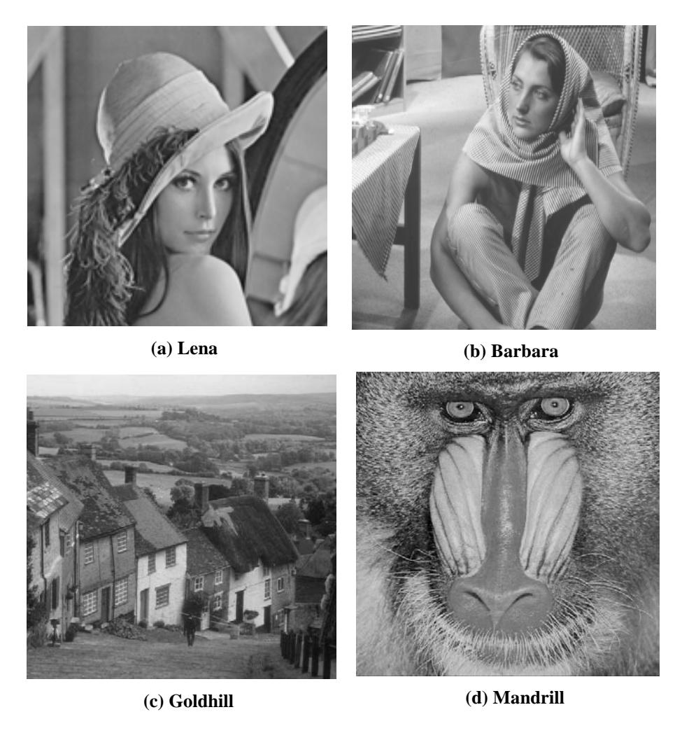
Figure 4 Grayscale (512×512) pixels test images.
The algorithm's rate distortion performance is represented by the peak signal to noise ratio (PSNR) measured in decibel (dB) vs. the compression bit rate defined as the average number of bits per pixel (bpp) of the compressed image. For 8 bpp grayscale images where the maximum pixel value is \(2^8 = 255\), the PSNR is given by:
\[PSNR = 10 \log_{10} \frac{255^2}{MSE} decibel (dB)\] (2)
where MSE is mean-squared error between the original image \(I_o\) and the reconstructed image \(I_p\) each with a size of M×N pixels, defined as:
\[MSE = \frac{1}{M \times N} \sum_{i=1}^{M} \sum_{j=1}^{N} [I_o(i,j) - I_r(i,j)]^2\] (3)
Another commonly used metric is the compression ratio (CR), which is the ratio of the size of the original image to the size of the compressed image, defined as [1,2]:
\[CR = \frac{\textit{Size of original image (Bytes)}}{\textit{Size of compressed image (Bytes)}} \tag{4}\]
For instance, CR = 50 means that the memory size of the compressed image is 50 times smaller than its original size after compression. Obviously, for any bit rate or CR, the highest PSNR is desired and for any PSNR, the lowest bit rate and highest CR is desired.
5.1 UFERS vs. other DWT-based Algorithms
In order to compare the proposed MSPECK to the wavelet-based SPECK and SPIHT algorithms, we used the DWT at the transformation stage and the transformed image was coded by MSPECK. For this purpose, we employed the bi-orthogonal 9/7 Daubechies 2D-DWT with 5 dyadic decomposition levels at the transformation stage for all algorithms. The initial set size for MSPECK was (128×128) pixels (Q = 8). Table 1 shows the PSNR versus bit rate and the compression ratio (CR) of the algorithms. The results of SPIHT and SPECK were taken from [14] because no arithmetic coding was used in the significance test or any symbols produced by the SPIHT or SPECK algorithms for these results, i.e. the output bits were written directly to the bitstream. In this way, the comparison is fair and meaningful. Arithmetic coding using contexts and joint encoding generally improves SPIHT and SPECK by about 0.5 dB but at the same time increases their complexities [10]. The table depicts the following:
- 1. SPECK had better PSNR than SPIHT for all images and bit rates.
- 2. The proposed MSPECK had slightly better PSNR for the "Lena" image, except at bit rate 2 bpp.
- 3. For the "Barbara" image, which has high-frequency content, the MSPECK outperformed SPECK for all bit rates.
- 4. MSPECK and SPECK had very similar PSNR for the "Goldhill" image.
These results indicate that the MSPECK and the SPECK algorithms have very similar PSNR. The advantage of MSPECK is the reduction of the memory requirements of the algorithm and the simplification of its memory management due to eliminating the array of the linked lists LISz that is used by SPECK.
Table 1 PSNR vs. Bit Rate and Compression Ratio (CR) for Gray-Scale (512×512) Pixels Test Images for the DWT-based SPIHT, SPECK, and MSPECK Algorithms.
| Image | Bit Rate (bpp) | 0.0625 | 0.125 | 0.25 | 0.5 | 1 | 2 |
|---|---|---|---|---|---|---|---|
| CR | 128 | 64 | 32 | 16 | 8 | 4 | |
| Lena | SPIHT | - | 30.25 | 33.46 | 36.68 | 39.88 | 44.15 |
| SPECK | - | 30.36 | 33.56 | 36.79 | 39.98 | 44.37 | |
| MSPECK | 27.72 | 30.65 | 33.67 | 36.80 | 39.98 | 44 | |
| Barbara | SPIHT | - | 24.39 | 26.92 | 30.71 | 35.78 | 41.82 |
| SPECK | - | 24.7 | 27.48 | 31.26 | 36.18 | 42.22 | |
| MSPECK | 23.67 | 25.16 | 28.02 | 31.99 | 37.05 | 43.43 | |
| Goldhill | SPIHT | - | 27.90 | 29.91 | 32.40 | 35.69 | 40.83 |
| SPECK | - | 28 | 30.13 | 32.71 | 36.01 | 41.13 | |
| MSPECK | 26.19 | 28.19 | 30.17 | 32.56 | 35.91 | 40.99 |
5.2 UFERS vs. other DCT-based Algorithms
In this subsection, we will compare the proposed DCT-based UFERS to the optimized JPEG [15], the DCT-based algorithm of Song, et al. [9] and the E-CEB of Tu, et al. [12]. In addition, a DCT version of SPIHT is also given, in order to depict the superiority of SPECK over SPIHT when used with DCT images. SPIHT was implemented using the public license program presented by Mustafa, et al. in [16]. For UFERS and DCT-SPIHT, the image was first DCT transformed using a block size of (16×16) pixels. The DCT coefficients were then rearranged into the dyadic wavelet structure before coding. Notice that a block size of (16×16) produces 13 subbands arranged in 4 wavelet decomposition levels. The initial set size for UFERS was (128×128) pixels (Q = 8). Table 2 shows the PSNR versus bit rate and the CR for the different DCTbased algorithms.
| Bit Rate (bpp) | 0.0625 | 0.125 | 0.25 | 0.5 | 1 | 2 | |
|---|---|---|---|---|---|---|---|
| Image | CR | 128 | 64 | 32 | 16 | 8 | 4 |
| UFERS | 26.76 | 29.62 | 32.92 | 36.37 | 39.69 | 44 | |
| Optimized JPEG | - | - | 32.30 | 35.90 | 39.60 | - | |
| DCT-SPIHT | 22.78 | 27.30 | 31.39 | 35.35 | 38.90 | 43.56 | |
| Lena | [9] | 27.57 | 30.28 | 33.36 | 36.64 | 39.93 | - |
| E-CEB | 26.82 | 29.83 | 33.16 | 36.63 | 40.08 | - | |
| MSPECK | 27.72 | 30.65 | 33.67 | 36.80 | 39.98 | 44 | |
| UFERS | 23.54 | 25.69 | 28.62 | 32.42 | 37.50 | 43.43 | |
| Optimized JPEG | - | - | 26.70 | 30.60 | 35.90 | - | |
| DCT-SPIHT | 21.01 | 23.63 | 26.93 | 30.87 | 36.30 | 42.4 | |
| Barbara | [9] | 24.06 | 26.43 | 29.27 | 32.82 | 37.52 | - |
| E-CEB | 22.73 | 24.99 | 27.83 | 31.91 | 36.98 | - | |
| MSPECK | 23.67 | 25.16 | 28.02 | 31.99 | 37.05 | 43.43 | |
| UFERS | 26.02 | 27.82 | 29.81 | 32.47 | 35.84 | 40.99 | |
| DCT-SPIHT | 22.87 | 26.35 | 28.98 | 31.71 | 35.07 | 40.01 | |
| Goldhill | [9] | 26.62 | 28.32 | 30.41 | 32.95 | 36.44 | - |
| E-CEB | 25.96 | 27.99 | 30.32 | 32.97 | 35.84 | ||
| MSPECK | 26.19 | 28.19 | 30.17 | 32.56 | 35.91 | 40.99 | |
| UFERS | 20.35 | 21.41 | 22.82 | 25.13 | 28.61 | 34.14 | |
| DCT-SPIHT | 19.13 | 20.52 | 22.23 | 24.46 | 27.97 | 33.53 | |
| Mandrill | [9] | 20.59 | 21.66 | 23.11 | 25.56 | 28.97 | - |
| MSPECK | 20.58 | 21.44 | 22.87 | 25.08 | 28.63 | 34.11 |
Table 2 PSNR vs. Bit Rate and Compression Ratio (CR) for Gray-Scale (512×512) Pixels Test Images for DCT Algorithms.
The table depicts the following:
- 1. DCT-SPIHT had the lowest PSNR among all algorithms. This is expected because as stated previously, SPIHT depends strongly on the self-similarity between the wavelet coefficients, which is a special feature of the dyadic 2D-DWT.
- 2. The proposed UFERS algorithm outperformed the optimized JPEG for all images and rates. As mentioned previously, the optimized JPEG uses Huffman coding, which is 4 times slower than the set partitioning approach that is adopted by UFERS. This means that UFERS is faster and more efficient than the optimized JPEG. In contrast, the algorithm of Panggabean from [13] was also faster than JPEG but it had lower efficiency.
- 3. The proposed UFERS algorithm is very competitive with DWT-MSPECK. The superiority of UFERS over MSPECK is the reduced complexity attained by using DCT instead of DWT.
- 4. The algorithm of Song [9] performed slightly better than UFERS. Unfortunately, the cost paid for this enhancement is the highly increased complexity since the complexity of the context-based arithmetic coder used by [9] is about (6-8) times higher than that the set partitioning technique used by UFERS or SPECK [10,15]. Consequently, this complexity increment reduces the low-complexity benefits of using DCT instead of DWT.
- 5. Compared to the E-CEB algorithm [12], which has about the same complexity as [9] as it also uses a context-based arithmetic coder, the UFERS had better PSNR for the Barbara and Goldhill images, which have high-frequency contents. This means that UFERS has better performance and has lower complexity than E-CEB.
It is worth noting that our UFERS algorithm is better than JPEG objectively (in terms of PSNR) as well as subjectively, where the reconstructed images are evaluated by viewers, due to the blocking artifacts of JPEG. This is depicted in Figure 5, which shows the Lena image decoded using UFERS (left) and the JPEG (right) at 0.25 bpp. As can clearly be seen, although both algorithms have about the same PSNR (≈ 32 dB), the UFERS is subjectively better.
(a) Decoded by UFERS (PSNR = 32.92) (b) Decoded with JPEG (PSNR = 32.3)
Figure 5 Lena image decoded at 0.25 bpp; (a) using UFERS; (b) using JPEG.
Finally, Table 3 shows the processing speed of the proposed MSPIHT and UFERS algorithms. The processing speed is represented as the average computer execution time for the four grayscale test images, measured in milliseconds (msec), of the compression and decompression processes against the compression bit rate. All algorithms were evaluated using C++ under a PC with Core i3, 1.8 GHz CPU and 2GB RAM. The compression time as well as the decompression time consists of a fixed time for the forward and reverse transformation stages, and a variable time for the coding and decoding processes that varies with the compression bit rate.
Table 3 Average Compression Time and Decompression Time vs. Bit Rate of Proposed MSPECK and UFERS Algorithms.
| Compression time (msec) | Decompression time (msec) | |||||
|---|---|---|---|---|---|---|
| Bit Rate (bpp) | MSPECK | UFERS | MSPECK | UFERS | ||
| 0.125 | 49 | 46 | 41 | 38 | ||
| 0.25 | 81 | 78 | 57 | 54 | ||
| 0.5 | 101 | 98 | 79 | 76 | ||
| 1 | 113 | 110 | 105 | 102 | ||
| 2 | 128 | 125 | 118 | 115 | ||
The following observations can be deduced from this table:
- 1. For all algorithms, the decompression time was shorter than the compression time due to their asymmetric property, since the decoder doesn't need to scan the sets' pixels at every bit-plane to see if the set becomes SIG.
- 2. UFERS was slightly faster than MSPECK due to using 2D-DCT instead of 2D-DWT. In addition, the difference in time was fixed (3 msec) because the transform time was fixed. It should be noted that the implemented DCT was not fully optimized for speed. In other words, the speed of DCT can be improved by using a fast DCT like the Fast Fourier Transform (FFT) [2].
The relation between the algorithm's performance and complexity is usually clarified by its performance to complexity ratio (PCXR), which is defined as the ratio between the algorithm's PSNR and the execution time that is needed to obtain this PSNR measured in dB/sec [17]. Evidently, a high PCXR with good PSNR is preferable. Table 4 depicts the average PCXR vs. the bit rate for the MSPECK and the UFERS algorithms at the encoder and decoder sides. The average PCXR represents the ratio of the average PSNR to the average execution time for the four test images. As can be seen, in spite of its (slightly) lower PSNR, the UFERS had a higher PCXR than MSPECK due to the speed advantage of DCT over DWT. In addition, the PCXR at the decoder was higher than that at the encoder for both algorithms due to their asymmetric property.
| Bit Rate | Average PCXR at Encoder | Average PCXR at Decoder | ||||
|---|---|---|---|---|---|---|
| (bpp) | MSPECK | UFERS | MSPECK | UFERS | ||
| 0.125 | 538 | 568 | 643 | 688 | ||
| 0.25 | 354 | 366 | 503 | 529 | ||
| 0.5 | 312 | 323 | 400 | 416 | ||
| 1 | 313 | 322 | 337 | 347 | ||
| 2 | 317 | 325 | 344 | 353 | ||
Table 4 Average Performance to Compression Ratio (PCXR) in dB/sec vs. Bit Rate of Proposed MSPECK and UFERS Algorithms.
In order to appreciate the superiority in processing speed of our algorithm over the algorithm of Song, et al. [9], it is given in [9] that the average encoding time of the algorithm is equal to 7.18 seconds evaluated using a Pentium 4 PC equipped with 2.4 GHz CPU, and 1 GB RAM. Unfortunately, the bit rate at which the encoding time was calculated and the employed programming language were not specified. However, assume that the encoding time in [9] was calculated at the worst case, where the bit rate was the highest possible rate and the programming language was Matlab (the slowest language). For the purpose of comparison, we have implemented our UFERS algorithm using Matlab too. The average encoding time at full rate was about 1.25 seconds, which indicates that the proposed UFERS is about 5 times faster than that of [9]. More importantly, at full bit rate, the average PSNR of UFERS was 38.45 dB, so the average PCXR was equal to 30.76 dB/sec. On the other hand, assuming that the average PSNR of [9] at full bit rate is 40 dB (a reasonable assumption (see Table 2), then the average PCXR is 5.57 dB/sec. This result is expected due the highly complexity of the sorting mechanism and the context-based arithmetic coding adopted by the algorithm of [9].
6 Conclusion
In this paper, we presented the UFERS algorithm. UFERS is a rate scalable algorithm that has good rate distortion performance and low computational complexity. The main contribution of the new algorithm is that it has the highest performance to complexity ratio among all current rate scalable algorithms. The speed advantage of the proposed algorithm makes it is very suitable for color image compression and real-time applications such as video transmission where compression speed is more important than efficiency. Furthermore, a fast algorithm requires short processing time and consequently it consumes less energy. This means that UFERS can be used with limited power devices such as mobile phones, digital cameras, etc. to preserve the life of the device's battery. Another advantage of UFERS over the algorithms from [9,12,13] is its asymmetric property as its decoding time is much faster than its encoding time. This asymmetric property is very valuable with scalable image
compression since the image is compressed only once and may be decompressed many times. Finally, the DC subband represents a thumbnail for the entire image or video frame. Thumbnails are very useful for fast image and video browsing, as only a rough approximation of the image or video is sufficient for deciding whether the image needs to be decoded in full or not. Thus, the proposed UFERS can be used with Web image and video browsers for fast browsing.