
1 Introduction
Path planning for mobile robots has been studied by researchers and practitioners to find optimal path planning solutions. Designing an optimal path is a difficult task [1,2]. There are many aspects that must be considered, such as the model of the environment, existing constraints, kinematics and the dynamic properties of the robot itself. These aspects should be identified carefully to yield efficient planning.
However, recent improvements in path planning have been developed to consider many factors such as the factors mentioned above and other factors such uncertainties, errors in modeling and optimality. Among these approaches, there is one common objective, i.e. finding the best and optimal trajectory. Some algorithms use a discrete and probabilistic approach [3] that is integrated with the basic theory of searching and dynamic programming with some minor changes [4,5].
Some researchers have developed path planning for mobile robots with cellular automata [6-9]. Cellular automata are a group of cells with a certain structure in which each cell has its own state, on or off. The state of the cell is able to change every time step according to a local rule with a simple arithmetic computation [10-13]. By exploiting the characteristics of the rule, the process of updating the states can be done efficiently with simple calculations.
An important part of planning design is optimization. In a static environment, the path is optimal if the distance is minimum. In a dynamic environment, the best path is not always the minimum path. Instead, we seek the path that guides the robot to the goal in the minimum amount of time without colliding with obstacles. In two previous works [8,9], we applied cellular automata to compute the shortest path between two points in a static environment. For the case of a dynamic environment, addressed in this paper, we expanded the cellular automata to cellular learning automata in order to optimize the path by exploring information from the environment. Cellular learning automata has been used before in other areas of problem optimization [14,16].
The main contribution of this study is to provide path planning alternatives for mobile robots using cellular learning automata. Existing path planning methods for mobile robots implemented in ROS (Robot Operating System) [17] were designed using Dijkstra's algorithm and the A* algorithm, where the path planning is computed step by step between two nodes of an irregular mesh. Our approach extends the existing method by exploiting the regularity of cellular automata in which the distance between two adjacent cells is equal. Furthermore, we use cellular learning automata to optimize the path generated in the first stage.
This paper is structured as follows: in Section 2, we review the theory of cellular automata, in Section 3 the path planning problem and its optimization are formulated, in Section 4 we discuss the complexity of the algorithm, in Section 5 we show our experimental results, and in the last section we conclude our work.
2 Cellular Automata
2.1 Two Dimensional Cellular Automata
Two-dimensional cellular automata are a group of cells in which one has a maximum of eight neighbors. There are two common structures, the von Neumann and Moore neighborhoods. These two models are distinguished by the number of neighbors. The von Neumann model has four neighbors while the
Moore model has eight neighbors. The Von Neumann and Moore models are shown diagrammatically in Figure 1.
Each cell in elementary cellular automata has two states, '0' or '1'. The state can change every time step when a local rule is applied. The next state of a cell at time t + I is affected by the state of its neighbors and its own state at time t.
Figure 1 Von Neumann model (left) and Moore model (right).
The state of the cellular automata is computed based on local rules. The local rule for two-dimensional cellular automata with von Neumann's neighborhood structure is defined as follows:
\[s_{i,j}^{(t+1)} = f\left[s_{i,j}^{(t)}, s_{i,j+1}^{(t)}, s_{i+1,j}^{(t)}, s_{i,j-1}^{(t)}, s_{i-1,j}^{(t)}\right] \tag{1}\]
The above rule can be expressed in another form, called totalistic, i.e. the sum of all neighbors, and is written as:
\[s_{i,j}^{(t+1)} = f \left[ s_{i,j}^{(t)} + s_{i,j+1}^{(t)} + s_{i+1,j}^{(t)} + s_{i,j-1}^{(t)} + s_{i-1,j}^{(t)} \right]\] (2)
It can also be written in a simple form:
\[C = \sum_{n} f(n)k^{n} \tag{3}\]
Each position of the cells is numbered, as shown in Figure 2. This numbering is used to compute the local rule. The rule for a cell with Moore's neighborhood structure is defined as the sum of the number of its neighbors.
| 64 | 128 | 256 |
|---|---|---|
| 32 | 1 | 2 |
| 16 | 8 | 4 |
Figure 2 Totalistic 2D cellular automata.
From Figure 2, for example, rule C = 170 (128 + 32 + 8 + 2) has only top, bottom, left, and right neighbors. Hence, in Moore's model, there are 512 rules. The rule for each cell can be similar (uniform) or different (hybrid).
2.2 Cellular Learning Automata
Cellular learning automata are cellular automata in which each cell has learning capability [14,16]. Such a cell is called a learning automaton. A learning automaton requires information from its environment to select the right action in order to get the best response. Each action has a certain probability, which will be updated regularly according to the response of the environment. The response type can be reward or penalty. A learning automaton interacts with its environment to collect the information, as shown in Figure 3.
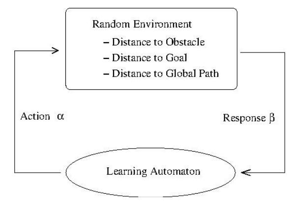
Figure 3 Interaction between a learning automaton and its environment.
2.3 Model of Environment
An environment is defined as a set of three tuples \(E = \{\alpha, \beta, p\}\), where
\(\alpha = \{\alpha_1, \alpha_2, \dots, \alpha_n\}\) : a set of actions \(\beta = \{\beta_1, \beta_2, \dots, \beta_n\}\) : a set of responses \(p = \{p_1, p_2, \dots, p_n\}\) : a set of probability of actions
The environment of type P has two kind of responses, \(\beta_1 = 1\): penalty and \(\beta_2 = 0\): reward. The components of the automata consist of four tuples \(\{\alpha,\beta,p,T\}\) where \(\alpha = \{\alpha_1,\alpha_2,...,\alpha_n\}\) is a set of actions, \(\beta = \{\beta_1,\beta_2,...,\beta_n\}\) represents the input, \(p = \{p_1,p_2,...,p_n\}\) is the probability of actions, and \(p(n+1) = T(\alpha(n),\beta(n),p(n))\) represents the local rule.
2.4 Updating Probability Action
The probability of actions is variable. If a learning automaton gets a reward, p increases and p of the other cells decreases. The probability of an action is updated according to the following rule:
If \[\beta = 0\]
\[P_i(n+1) = P_i(n) + a[1 - P_i(n)]\] \[P_i(n+1) = (1 - a)P_i(n) \,\forall i, j \neq i\] (4)
If \(\beta = 1\)
\[P_{i}(n+1) = (1-b)P_{i}(n)\] \[P_{j}(n+1) = \frac{b}{r-1} + (1-b)P_{j}(n) \,\forall j, j \neq i\] (5)
where a and b are parameters of reward and penalty respectively.
3 Problem Formulation
In this paper, we use two-dimensional cellular automata with Moore's neighborhood structure, i.e. there are eight neighbors for each cell. Each cell interacts with its nearest neighbors, as shown in Figure 4. The distance between two cells is computed based on the Manhattan rule.
Figure 4 Model of two-level interaction.
3.1 Computing Global Path
Let \(N_i^t\) be the neighborhood of cell i at time step t, and \(s_i^t\) the state of cell i. This state represents the distance to the goal. The rule to compute the distance to the goal is defined by:
\[s_i^{t+1} = \begin{cases} \min\{s_x^t\} + 1 \text{ if } s_i^t \text{: a free cell, } s_x^t \text{: are filled cell, } s_x^t \in N_i^t \\ s_i^t & \text{if } s_i^t \text{: is not a free cell} \end{cases}\] (6)
The above rule maintains the minimum distance to the goal because it always selects the cell in the neighborhood with the minimum state. Therefore, the distance from any point to the goal will be minimum.
3.2 Optimizing Local Planning
The distance between the initial position and the goal position needs to be recomputed when new obstacles arise. In this case, the global path is modified to adapt to the change. In this process, we consider three variables that will influence the overall performance and particularly the total distance to the goal.
- 1. The obstacle variable indicates the proximity to the obstacles. It is denoted by \(c_{obs}(i,j)\), i,j=1,2,...,N.
- 2. The goal variable indicates the distance to a goal position that is obtained from the global path. It is denoted by \(c_{goal}(i,j)\), i,j=1,2,...,N.
- 3. The path variable indicates the distance to the nearest global path. It is denoted by \(c_{path}(i,j)\), i,j=1,2,...,N.
3.3 Cost Function
In this model, we have to minimize the objective function of the three distance variables. A small value of the first variable shows that the robot's position is farther from the obstacle, whereas the second and the third variable show the remaining distance to the goal and the global path. The cost function is defined as follows:
\[\operatorname{Min} F(C) = \sum_{\substack{i=i_0 \\ N_{goal}}}^{N_{goal}} \sum_{\substack{j=j_0 \\ N_{goal}}}^{N_{goal}} w_{obs} c_{obs}(i,j) + \sum_{\substack{i=i_0 \\ j=j_0}}^{N_{goal}} \sum_{\substack{j=j_0 \\ w_{path}}}^{N_{goal}} c_{goal}(i,j) +\] \[\sum_{\substack{i=i_0 \\ j=j_0}}^{N_{goal}} \sum_{\substack{j=j_0 \\ j=j_0}}^{N_{goal}} w_{path} c_{path}(i,j)\] \[(7)\] where:
\(N_{goal}\): the number of steps required to reach the goal.
: the weighting factor of the obstacle variable.
: the weighting factor of the goal variable ℎ : the weighting factor of the path variable
, , ℎ ∈ , , = 1,2, … , .
As given in Eq. (7), the cost function that is represented as the weighted sum of the three selected variables must be minimum in order to obtain the optimal path.
3.4 Updating Individual Cells
Each cell is updated according to the following rule and the next cell will be selected from its neighbors with the minimum value.
\[\Delta F(c(i,j)) = \sum_{m} f_{obs}(c(k,l), p_{ij}(k,l), w_{obs}) +\] \[\sum_{m} f_{goal}(c(k,l), p_{ij}(k,l), w_{goal}) + \sum_{m} f_{path}(c(k,l), p_{ij}(k,l), w_{path})\] (8)
where:
(,) : cost at cell (i,j).
(, ) : probability to select cell (k,l) from cell (i,j).
If there is no penalty in the learning scheme, then the probability is updated as follows:
\[p_{ij}(t+1) = \begin{cases} p_{ij}(t) + a(1 - p_{ij}(t)) & \text{if } c_{ij}(t) < c_{kl}(t) \\ p_{ij}(t) & \text{otherwise} \end{cases}\](9)
\[p_{ij}(k,l)(t+1) = \begin{cases} p_{ij}(k,l)(t) - a \, p_{ij}(k,l)(t)), & \text{if } c_{ij}(t) < c_{kl}(t) \\ p_{ij}(k,l)(t) & \text{otherwise} \end{cases}\](10)
The reinforcement signal, defined as () = { : = 1,2, … , }, is positive (+1) if () < () and is negative (-1) if () ≥ ().
3.5 Initial Probability Action
Initially, p is assigned a certain value. We can use one of the following rules. In this case we use Rule 3, in which the cell with the minimum cost will be the best candidate cell.
- 1. The value of p is set to 1/m for all cells.
- 2. The value of p is set to 0 or 1 as follows:
\[p_{ij}(k,l) = \begin{cases} 1, & p_{ij}(k,l) = \max_{c(k,l) \in N(c(i,j))} \{p_{ij}(k,l)\} \\ 0 & \text{otherwise} \end{cases}\] (11)
3. The value of p is computed from the cost function. If the value of c is small, the value of p is large according to the following relation,
\[p_{ij}(k,l) = \frac{(1/c(k,l))}{\sum_{m} 1/N(c(i,j))}, \qquad c(k,l) \neq c(i,j),\] \[c(k,l) \in N(c(i,j))\] (12)
where: N(c(i,j)) : neighbors of c(i,j)
4 Complexity
The path is determined using a backward search algorithm. As long as the initial position and the goal position are not in an area surrounded by obstacles, the goal position is reachable from the initial position. Hence, the algorithm is complete. The cost required to execute the algorithm depends on the size of the cells. If the size of the environment is \((x_{max} \times y_{max})\), then the number of steps required is:
\[(x_{max} \times y_{max})(a+m) \tag{13}\] where:
a: the number of access, read and write operations.
m: the number of neighbors.
The number of steps from initial to goal position is used to measure the distance. We assume the distance is computed based on the Manhattan rule. The number of steps is \((x_{max} \times y_{max})(a+m) \times d\), where d is the distance from the initial position to the goal position. The worst case occurs if d approaches \((x_{max} \times y_{max})/2\), and the number of steps is:
\[(x_{max} \times y_{max})(a+m)(x_{max} \times y_{max}) \tag{14}\]
Hence, the order of the algorithm is \(O(x_{max}^2 \times y_{max}^2)\), which is the same order as Dijkstra's algorithm without min-priority queue, that is \(O(|V|^2)\), where |V| is the number of vertices. If a global path is given, the number of steps required is
(a + m) × d × l in the worst case and (a + m) × d in the best case, and l is the level of interaction.
5 Experiments
In this experiment we define the environment as the model of a building with many rooms and the number of robots is 1, as shown in Figure 5. Before the robot makes explorations, it creates a map of the environment as shown in Figure 6-8. The map is used to determine the global path. The global paths generated by two different planning are shown in Figure 6-8. The first global path is generated using cellular automata in which the distance is computed using the Manhattan rule, while the second path is generated based on Dijkstra's algorithm.
Figure 5 The model of environment.
In this experiment, we use a model of a mobile robot, Pioneer3AT, and the Gazebo simulator [18] to model the environment. The robot is controlled by programs executed in an ROS environment. The programs execute global and local path planning, implemented using cellular automata. The program works as follows. Initially, the global path is generated and the robot starts to move along it. Then, the local path planning is activated to update the global path if required, for example if the global path is blocked by new obstacles such that it is not available anymore. The program will stop when the robot reaches the goal position.
The results of the experiment with global path planning are shown in Figures 6- 8. The first path, generated using cellular automata, was closer to the obstacles than the second one, which was generated using Dijkstra's algorithm. However, it generated more segments than Dijkstra's algorithm.
Figure 6 Global path to Goal I generated using cellular automata (left) and Dijkstra's algorithm (right).
Figure 7 Global path to Goal II generated using cellular automata (left) and Dijkstra's algorithm (right).
Figure 8 Global path to Goal III generated using cellular automata (left) and Dijkstra's algorithm (right).
The performance of local path planning is determined by the cost function as defined in Eq. 7. Here, we set the weighting factor for all distance variables as follows: = 0.06, = 0.08, ℎ = 0.01. The central cell of the cellular automata interacts with its neighbors at Level 1 and Level 2 as shown in Figure 4. The map resolution is 0.05 measured in meters and the granularity of the cells is 0.05. Details of the simulation results are shown in Table 1.
In the other experiment we computed the global path of 3 robots using three existing algorithms, Dijkstra's algorithm, the A* algorithm and the Cellular Learning Algorithm (CLA). A standard algorithm was used for the purpose of comparison. The global paths generated using the three algorithms are shown in Figures 9 and 10.
| Table 1 Simulation results for three different goals. |
|---|
| goal-1 | goal-2 | goal-3 | |||||
|---|---|---|---|---|---|---|---|
| dijks | cla | dijks | cla | dijks | Cla | ||
| Initial | (-8,-5) | (-8,-5) | (-8,-5) | (-8,-5) | (-8,-5) | (-8,-5) | |
| Goal | (8,-14) | (8,-14) | (0,5) | (0,5) | (-8,4) | (-8,4) | |
| Direct-Dist | 744 | 745 | 515 | 515 | 356 | 356 | |
| Path-Len | 788 | 840 | 689 | 632 | 621 | 582 | |
| Times in sec. | 64.4 | 77.2 | 52.6 | 58.8 | 48.2 | 59.8 | |
Figure 9 Global path of three robots generated using Dijkstra's algorithm (left) and the A* algorithm (right).
Figure 10 Global path of three robots generated using CLA.
The global path generated using CLA was similar to that generated using Dijkstra's algorithm; the difference is not significant. The difference of the path occurs when the robots are moving, in this case when the local path planning is active. Details of the results are shown in Table 2.
Table 2 Performance of three robots.
| Parameter | Dijkstra | A* | CLA | ||||||
|---|---|---|---|---|---|---|---|---|---|
| Rob1 | Rob2 | Rob3 | Rob1 | Rob2 | Rob3 | Rob1 | Rob2 | Rob3 | |
| 1. Start pos. | -8,-5 | -8,-4 | 5,4 | -8,-5 | -8,-4 | 5-4 | -8,-5 | -8,-4 | 5,4 |
| 2. Goal pos. | -2,-13 | -2,-14 | -2,-15 | -2,-13 | -2,-14 | -2,-15 | 2,-13 | -2,-14 | -2,-15 |
| Parameter | Dijkstra | A* | CLA | ||||||
|---|---|---|---|---|---|---|---|---|---|
| Rob1 | Rob2 | Rob3 | Rob1 | Rob2 | Rob3 | Rob1 | Rob2 | Rob3 | |
| 3. Path to R1 | - | 655 | 755 | - | 704 | 796 | - | 564 | 594 |
| 4. Path to R2 | 662 | - | 669 | 649 | - | 670 | 570 | - | 626 |
| 5. Path to R3 | 727 | 610 | - | 814 | 684 | - | 594 | 524 | - |
| 6. Path R1-G | 480 | 503 | 520 | 486 | 549 | 589 | 550 | 550 | 550 |
| 7. Path R2-G | 931 | 951 | 1004 | 861 | 882 | 941 | 922 | 904 | 922 |
| 8. Path R3-G | 881 | 918 | 953 | 902 | 9 | 982 | 850 | 850 | 850 |
| 9. Path to G | 480 | 951 | 953 | 486 | 882 | 982 | 550 | 904 | 850 |
| 10. Dist to G | 408 | 738 | 813 | 408 | 738 | 813 | 408 | 738 | 813 |
| 11. Maze level | 1.176 | 1.288 | 1.172 | 1.191 | 1.195 | 1.208 | 1.348 | 1.225 | 1.046 |
| 12. Time to G | 63.6 | 128.8 | 164.0 | 63.4 | 132.4 | 135.4 | 62.4 | 116.0 | 156.6 |
Note: the map resolution is 0.025; 1 unit coordinates = 40 steps (path length)
Three parameters were used as a measure of performance: path length, total time to the destination, and complexity of the path. The complexity of the path is defined as the ratio between the actual path length and the direct distance to the destination assuming there are no obstacles on the way to the destination. Path length is a suitable parameter if the environment is static, otherwise total time is a better choice to measure performance. The path length is also influenced by the algorithm used. Using the three different algorithms in these experiments, the resulting trajectories had different lengths. Dijkstra's algorithm had the shortest trajectory, then the A* algorithm, and the longest was CLA's. In fact, Dijkstra's algorithm does not turn frequently and does not emphasize the shortest distance to the nearest obstacle. On the other hand, CLA generates a path that is straight, because the curves follow the shape of the obstacles and it emphasizes the closest distance to the obstacles.
Total time is a measure of the actual time it took the robot to reach the goal position. In the case of a dynamic environment, total time is a suitable choice to measure performance. From the experimental results, the best performance based on total time measurement was CLA, then the A* algorithm, and the worst was Dijkstra's algorithm.
The last parameter is the complexity of the path (maze level). The greater the number, the more twists and turns in the trajectory were generated. From the experimental results, Dijkstra's algorithm had the lowest maze level, then the A* algorithm, and the highest one was CLA's.
6 Conclusion
Path planning for mobile robots can be implemented efficiently with cellular automata. Its computational process is suitable for being implemented on lowcost hardware such as an on-board computer or microcontroller that is integrated with the robot. By using cellular automata, the process of updating the states to select the optimal path can be done in parallel due to the asynchronous properties of the cells.
In the second stage of planning, CLA is used to handle the dynamic properties of the environment. In comparison with existing algorithms, such as Dijkstra's algorithm and the A* algorithm, the algorithm with learning automata (CLA) is able to produce a path that stays closer to the obstacles and has a shorter travelling time than other two. However, it also causes the robot to turn frequently and produce straight segments along the whole path.
Acknowledgements
We gratefully acknowledge the support for this work by the Ministry of Higher Education of Indonesia through BPPS scholarships.