
1 0BIntroduction
Electrical capacitance volume tomography (ECVT) is a further development of electrical capacitance tomography (ECT), which is used for volumetric imaging. In ECT, the reconstruction of a 3D object is done by stacking 2D imaging slices [1]. ECVT, on the other hand, is able to reconstruct 3D objects directly. Thus, for more rapid observation, ECVT is more reliable compared to ECT.
The imaging technique and the image reconstruction algorithm are among the most important issues in improving ECVT performance beside the data
acquisition technology. The soft-field properties of electrical based tomography and the ill-conditioned measurement matrix are crucial factors that make the inverse problem (ECVT imaging) difficult to solve. The reconstruction algorithms that so far have been implemented in ECVT are ILBP [2], NN-MOIRT [2] and Combined Feed Forward NN and ILBP [3]. ILBP, or the Landweber algorithm, is one of the oldest methods for electrical based tomography, including ECT. It will always be a benchmark for all proposed imaging methods due to its simplicity and acceptable imaging performance in simple cases.
The most current reports show that NN-MOIRT performs much better compared to ILBP, especially when conducting dynamic observation [2]. When ILBP is applied, elongation noise is still observed for both static and dynamic ECVT imaging [2], while NN-MOIRT is successful in reducing it. In addition, in dynamic observation NN-MOIRT is successful in providing more stable imaging [2]. However, like all neural network based methods, NN-MOIRT is expensive in computational cost.
The compressive sensing framework is a new concept of signal recovery that enables the recovery of a certain signal that is naturally sparse or sparse in a certain domain by having a number of linear projections with a dimension that is considerably lower than the number of samples required by the Shanon-Nyquist Theorem [4-6]. The ECVT signal is naturally sparse and the dimension of capacitance measurement is much lower compared to the number of permittivity projections. Thus, theoretically, the compressive sensing framework is promising for adaption to ECVT imaging.
This paper discusses the possibility of developing an ECVT imaging technique based on the CS framework. It discusses the crucial part of adapting CS and presents the future potential of CS framework ECVT imaging techniques based on an early simulation of non-optimized compressive sensing for ECVT imaging and a number of previous scientific reports. Based on the simulation results, Non-optimized CS was not completely successful in providing better ECVT imaging quality. However, it did provide more localized imaging compared to ILBP and potentially provides a smaller number of electrodes required. In addition, the CS framework mathematically has high potential to be further developed and optimized for ECVT imaging by considering the high undersampling of ECVT and the structure of the ECVT projection matrix.
2 ECVT (Electrical Capacitance Volume Tomography)
ECVT is a tomography technique based on capacitance measurement. It is used to predict the permittivity distribution inside the sensing domain utilizing
capacitance measurement on the sensor boundary [2,7,8]. The technique, originally invented by Warsito, et al. [2], is a further development of ECT, which is used for volumetric imaging. The technique is able to do 3D object imaging directly, which makes it more reliable for rapid observation compared to ECT [2].
The basic difference between ECT and ECVT can be seen clearly when it comes to producing a reconstruction of a 3D object. 3D reconstruction by ECT projection is generated by stacking slices of 2D images. In ECVT, the reconstructed 3D image is generated directly without stacking procedure and it can be done in real time [2]. To produce a 3D reconstruction, ECVT utilizes the fringe effect, which is dependent on the sensor design [2].
2.1 ECVT Component
There are three main hardware components that support the ECVT system, i.e. the sensoring system, the data aqcuisition system, and a computer system for image reconstruction.
Figure 1 ECVT hardware components (Source: CtechLab).
The sensoring system consists of electrodes that produce capacitance excitation between electrode couples. For a number N of installed electrodes there are N(N-1)/2 possible capacitance measurements [2]. The data acquisition system processes the capacitance and electrical field measurements to prepare them for processing by the computer system. The computer system consists of algorithms that utilize the measurements to build the reconstructed image. The corresponding reconstructed image describes a prediction of the permittivity distribution inside the sensing domain.
Currenly, ECVT is not only being utilized in process tomography but also for medical tomography [9,10]. Edawar Technology have developed and implemented ECVT for breast and brain tomography. Thus, the architecture of ECVT sensor design various subject to the tomography purposes.
2.2 Mathematical Model
As a working process (software), the ECVT system consists of two main parts: the forward problem and the inverse problem. The forward problem covers the capacitance measurement on the sensing boundary and the inverse problem covers the prediction of the permittivity distribution inside the sensing domian utilizing the capacitance measurements.
2.1.1 Forward Problem
The basic forward problem of ECVT, the same as defined for ECT, is the capacitance measurement process that follows the Poisson equation that can be represented in a 3-dimensional space as in Eq. (1) [2,9,11]:
\[\nabla \epsilon(x, y, z) \nabla^2 \phi(x, y, z) = -\rho(x, y, z) \tag{1}\] where \(\nabla \epsilon(x, y, z)\) represents the permittivity distribution, \(\nabla^2 \phi(x, y, z)\) represents the potential distribution of the electrical field and \(\rho(x, y, z)\) represents the charge density. By assuming there is no charge inside the sensor, Eq. (1) can be represented as [2]:
\[\nabla \epsilon(x, y, z) \nabla^2 \phi(x, y, z) = 0 \tag{2}\]
Due to Eq. (2), the potential value can be calculated by the finite element method (FEM). If the potential can be calculated, then the capacitance can be calculated by the volume integral below[2]:
\[C_i = -\frac{1}{\Delta V_i} \oint_{A_i} \epsilon(x, y, z) \nabla \phi(x, y, z) dA\] (3)
where \(\Delta Vi\) is the voltage difference between the electrode pair and Ai is the surface area enclosing the detector electrode. Eq. (2) relates the dielectric constant (permittivity) distribution inside the sensing domain, \(\epsilon(x, y, z)\), to the measured capacitance, \(C_i\).
The linearization method, called the sensitivity model, is used to approach the solution of the forward problem given in Eq.(3). The linearization method is chosen due to its simplicity. The linearized form of Eq. (3) is mathematically formulated as in Eq. (4) [2]:
\[C = SG \tag{4}\] where C is the M-dimension of the measured capacitance vectors, G is the Ndimension of the permittivity distribution vector and S is the M x N dimension of the sensitivity matrix.
2.2 Inverse Problem
The inverse problem of the ECVT system is the process of utilizing the measured capacitance along the boundary to predict the permittivity distribution, \(\epsilon(x, y, z)\), inside the sensing domain. By having a linearized model of the capacitance-permittivity relation as given in Eq. (4), the inverse problem can be formulated mathematically as:
\[G = S^{-1}C \tag{5}\]
Eq. (5) seems simple to solve. However, the dimension of the predicted permittivity distribution (N) is normally much higher compared to the dimension of the measured capacitance (M). The problem in Eq.(5) becomes illposed or the system has an undetermined solution. This is a main issue in the image reconstruction research area, especially in electrical tomography.
3 Compressive Sensing Framework
Compressive sensing (CS) is a developing framework that was first formulated mathematically by Danoho, et al. [4] in 2004-2006. It states that any signal that is naturally sparse or sparse in a certain domain can be exactly recovered from the number of signal samplings of which the dimension is considerably lower than the number of samplings required by the Shanon-Nyquist theorem [4,12]. Mathematically, this concept is another approach of solving a linear system that has a smaller number of equations compared to the number of variables that should be solved, which is called an undetermined linear system.
3.1 Mathematical Model
Given a discrete time signal \(x \in \mathbb{R}^N\) and considering a measurement system that acquires M-dimension of measurement values, then mathematically the linear measurement can be represented as in Eq.(6) [6,12]:
\[y = \Phi x \tag{6}\] where \(\Phi \in \mathbb{R}^{M \times N}\) and \(y \in \mathbb{R}^{M}\). \(\Phi\) represents the measurement or sensing matrix. Mis typically much smaller compared to N. \(x \in \mathbb{R}^N\) is a coefficient vector that normally has only \(K \ll N\) non-zero coefficients [6,12]. In order to ensure that the original signal is properly adapted to the compressive sensing, the original signal x is often reformulated as a linear combination of a small number of signals taken from a 'resource database' determined as dictionary \(\psi \in \mathbb{R}^{N \times L}\)
[5,6]. The elements of the dictionary are typically unit norm functions called atoms [6].
\[x = \psi s \tag{7}\]
Then x in Eq.(7) is determined as a sparse signal in base \(\psi\) with K-degree of sparseness.
By representing the original signal in a certain dictionary, the linear measurement on Eq. (6) can be represented as:
\[y = \Phi \,\psi s \tag{8}\]
The main idea of the CS system is projection of x to a low-dimensional measurement vector y by measurement matrix \(\Phi\), which completely has no relation to sparse base \(\psi\) [5, 12]. However, some mathematical works and former simulations have shown criteria that should be satisfied by the measurement matrix in correlation with the sparse base matrix to achieve good CS performance.
The mathematical model given in Eq. (8) indicates that the measurement matrix and the sparse base (dictionary) matrix are crucial parameters in the CS system. Thus, most of the algorithms proposed for improving the CS system performance provide an optimization procedure for both of these parameters [6, 13-16].
3.2 Fundamental Compressive Sensing Principles
A number of references present fundamental compressive-sensing principles concerning aspects that affect compressive sensing performance. By acknowledging these properties, optimal performance of compressive sensing should be achieved. Two fundamental principles that should be addressed to optimize CS performance are sparsity and the incoherence principle.
3.2.1 Sparsity
In a compressive sensing framework, the recovery of a signal can be exact if the signal being sensed has a low information rate [6,12]. In other words, it is sparse in the original or another, transformed domain. Thus, sparsity is one of the crucial properties in the compressive sensing framework. Normally, to make sure that the sparsity of the signal is reliably adaptable to the compressive sensing framework, the sensed signal is transformed to a certain domain by a certain sparse base function that is called a dictionary [5]. Some commonly used dictionaries are the cosine base, the sine base, the wavelet base, the chirplet base, the curvelet base function, etc. [5].
3.2.2 Incoherence
The second most important principle of the CS framework in achieving optimal performance is the incoherence principle. The more incoherence between the measurement matrix and the dictionary, the more optimal recovery should be. Mathematically, the incoherence principle is represented by the restricted isotropy property (RIP).
3.2.2.1 Restricted Isotropy Property
The restricted isotropy property is a property that should be satisfied by measurement matrix Φ to guarantee the convergence of the reconstruction algorithm that recovers any K-sparse signal using M measurement values [4- 6,12]. Mathematically, for any K-sparse signal and any constant ∈ (0,1), the RIP criterion restricts the Φ, to the following criteria in Eq. (9) [5]:
\[1 - \varepsilon \le \frac{\|\Phi \psi s\|_2}{\|s\|_2} \le 1 + \varepsilon \tag{9}\]
The interpretation of the above criterion is the un-correlation (incoherency) between the measurement matrix and the sparse base matrix (dictionary).
Another way to see the un-correlation between the measurement matrix and the sparse base matrix is by observing the mutual coherence between these two parameters using the Gram matrix.
3.2.2.2 Mutual Coherence
Mutual coherence of = Φ , denoted as (), determines the worst-case coherence between any two columns (atoms) of A [17].
Definition 1 For a given matrix = Φ , the mutual coherence of A {()} is defined as the largest absolute and normalized inner product between the two different columns in A, formulated as in Eq.(10) [18]:
\[\mu(A) \cong \max_{1 \le i \ne j \le L} \frac{|A_i^T A_j|}{\|A_i\|_2 \|A_j\|_2}\] (10)
The strongest similarity between the different columns of matrix A can be evaluated by their mutual coherence. The measurement can reflect the weakness of the matrix. A close relationship between two columns may confuse any greedy pursuit algorithm, which can lead to inappropriate reconstruction [18].
The Gram matrix is considered another way to measure mutual coherence.
Definition 2 For a given matrix = Φ , the Gram matrix is defined as in Eq. (11) [6]:
\[G = A^T A (11)\] the (i,j)-th element of the Gram matrix of A is defined as in Eq. (12)[6]:
\[g_{ij} = A_i^T A_j \tag{12}\]
The Gram matrix is normalized such that = 1, ∀ = . The mutual coherence of A is determined by the maximum value of the off-diagonal elements of G.
The values of the mutual coherence are bounded in the interval of ≤ () ≤ 1, with low bound defined as in Eq.(13) [6]:
\[\underline{\mu} \cong \sqrt{\frac{L-M}{M(L-1)}} \tag{13}\]
Instead of the maximum value of the off-diagonal elements of G, the former simulations show that the average of the mutual coherence is more related to the performance of the CS system. Thus, the other measurement, called average mutual coherence, is drawn as in Eq. (14) [6]:
\[\bar{\mu}(A) = \frac{\sum_{\forall (i,j), with \ i \neq j} g_{ij}}{N_t}\] (14)
with off-diagonal elements. In this paper, the distribution of the off-diagonal entries of normalized Gram matrix G is presented to give a supporting reasons for the resulted simulation performance.
4 Non-Optimized Compressive Sensing Framework for ECVT Imaging
An early simulation of implementing a non-optimized CS framework for ECVT imaging is presented in this paper. The simulation's aim was to show the nature performance of the CS framework for ECVT imaging without optimizing the incoherency between the measurement matrix and the corresponding dictionary. The performance of the algorithm in terms of ECVT imaging quality was observed, so that the future potential of ECVT imaging based on the CS framework can be proposed.
4.1 The Framework for ECVT Imaging
The compressive sensing framework on ECVT imaging can be correspondingly explained as represents the measuring capacitance (c), Φ represents the sensitivity matrix (S), and x represents the permittivity distribution (g). Thus, Eq. (6) can be represented as in Eq. (15):
\[c = Sg \tag{15}\]
By representing the signal of the permittivity distribution as a sparse signal in a certain dictionary \(\psi\), permittivity distribution g can represented as in Eq.(16):
\[g = \psi \alpha \tag{16}\]
Thus, the linear capacitance measurement along the sensor's boundary can be represented as in Eq. (17):
\[c = S \psi \alpha\] (17)
\(\alpha\) is sparse, thus theoretically Eq. 17 should have an exact solution. The sparse signal \(\alpha\) can be obtained by Eq. (18) [5]:
\[\min \|\alpha\|_{l_0} \quad s.t \quad c = S \ \psi \alpha \tag{18}\]
The image reconstruction technique in the compressive sensing framework will find the optimum predicted sparse signal representation \(\alpha\) that correspondingly will obtain the optimum predicted permittivity distribution g by Eq. 16.
The Algorithm of ECVT Imaging by Non-Optimized CS 4.2
Step 1 (Data acquisition)
Data acquisition intends to obtain the capacitance measurement, the sensitivity approximation, and their corresponding normalization. The sensitivity is approximated by Eq. (19)[2]:
\[S_{ij} \cong V_{0j} \frac{E_{si}(x,y,z).E_{di}(x,y,z)}{V_{si}V_{di}}\] \[\tag{19}\] where \(E_{si}(=-\nabla\phi)\) is the electrical field distribution vector when the source electrode in the ith pair is activated with voltage \(V_{si}\) while the rest of the electrodes are grounded. \(E_{di}\) is the electrical field distribution vector when the detector electrode in the ith pair is activated with voltage \(V_{di}\) while the rest of the electrodes are grounded. \(V_{0,i}\) is the volume of the jth voxel.
Step 2 (Sparse base (dictionary) determination)
Determine the dictionary (sparse base) that will represent the original signal g in a certain sparse domain. In this early simulation, an orthogonal DCT (discrete cosine transform) base was used. If the length of the original signal is N, the orthogonal DCT base can be written as in Eq. (20):
\[\psi(m,n) = \sqrt{\frac{2}{N}} \left[ c(m)\cos\frac{(2n-1)(m-1)}{N} \right]\] (20)
where
\[m, n = 1, 2, ..., N, \ c(m) = \begin{cases} \frac{1}{\sqrt{2}}, \ m = 1\\ 1, \ m = 2, 3, ..., N \end{cases}\]
Step 3
Solving the optimization problem on Eq.(18) in order to obtain the representing sparse signal α. In this early simulation, a classical greedy iterative, orthogonal matching pursuit (OMP) algorithm is applied.
Step 4
Calculate the prediction of the original signal based on Eq. (16).
4.3 Simulation Set-up
To evaluate the performance of the proposed algorithm, we used syntactic data generated by Comsol. Static object simulation with various dielectric contrasts was designed. The simulation employed Comsol and MATLAB as the main software. A flow diagram of the corresponding simulation is shown in Figure 2.
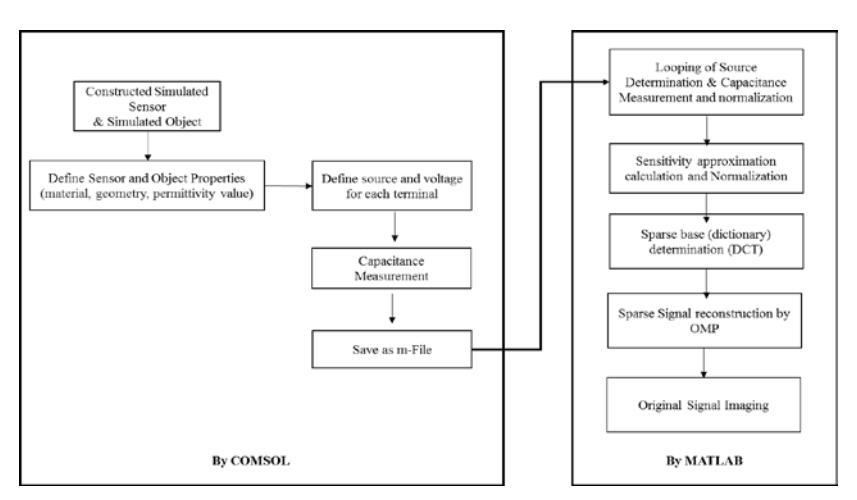
Figure 2 Flow diagram of simulation.
Comsol was utilized to replace the experimental set-up. It can be used to imitate the physical behavior during the sensing process by ECVT. The sensor design, detected object design and all corresponding properties were set up in Comsol. In addition, the capacitance and the electrical field measurement for the first activated port were simulated in Comsol, while the remainder was done by creating routines in MATLAB. Sensitivity approximation calculation, dictionary determination and the imaging process were done by writing the codes in MATLAB.
The used sensor design was a cylindrical sensor with 8 electrodes, as shown in Figure 3.
Figure 3 Cylindrical sensor with 8 electrodes, d = 10 cm, h = 20 cm, (Source: CTech Lab).
Detailed specifications of all properties used in the simulation are presented in Table 1. The simulation's properties covered the sensor geometry, shape and position of the detected object, contrast dielectric value, and the performance parameter used to measure the imaging performance.
Table 1 Properties of simulation.
| Simulation's Properties | Specification |
|---|---|
| Sensor geometry | Cylindrical sensor with 8 electrodes |
| Detected object | Ball with r = 4 cm |
| Dielectric contrast | 1:3; 1:6; 1:80 |
| Detected object position | Center of the sensor |
| Number of objects detected | Single object |
| Performance measurement parameter | Visual observation, NMSE, NMAE, R |
5 Simulation and Discussion
The simulation represents the performance of a non-optimized CS framework for ECVT imaging. The ILBP (Landweber) algorithm was used as benchmark. Visual observation and a number of quantitative measurements, coefficient of correlation (R), normalized mean square error (NMSE) and normalized mean absolute error (NMAE), were used to evaluate the performance of ILBP and Non-optimized CS for ECVT imaging. Both of the simulations of ILBP and Non-optimized CS used a 20 x 20 x 20 resolution.
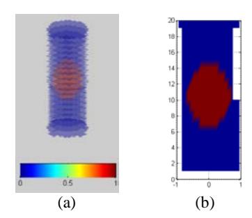
Figure 4 Actual imaging.
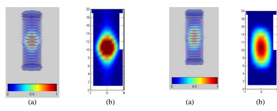
Figure 5 ILBP; contrast dielectric 1:3.
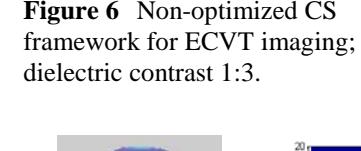
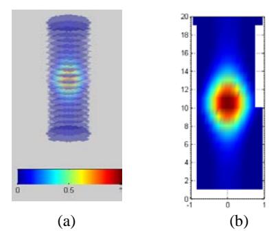
Figure 7 ILBP; dielectric contrast 1:6.
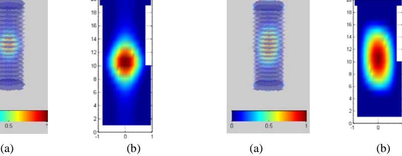
Figure 8 Non-optimized CS framework for ECVT imaging; dielectric contrast 1:6.
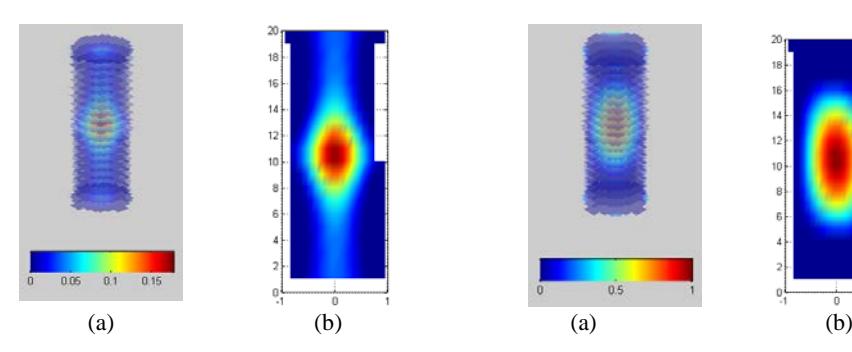
Figure 9 ILBP; dielectric contrast 1:80.
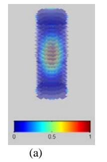
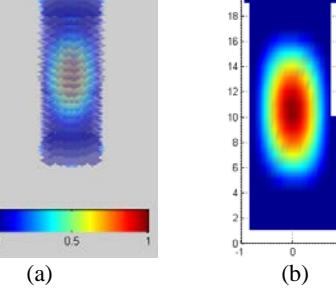
Figure 10 Non-optimized CS framework for ECVT imaging; dielectric contrast 1:80.
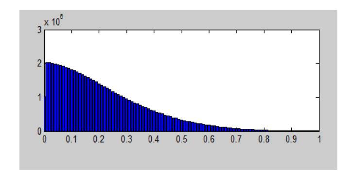
Figure 11 Off-diagonal component distribution (Gram matrix).
Table 2 Quantitative performance measurement.
| ILBP | Non Optimized CS | |||||
|---|---|---|---|---|---|---|
| 1:3 | 1:6 | 1:80 | 1:3 | 1:6 | 1:80 | |
| NMSE | 0.0274 | 0.0296 | 0.0387 | 0.0263 | 0.0263 | 0.0253 |
| NMAE | 0.7837 | 0.7835 | 0.9683 | 0.7941 | 0.7911 | 0.8902 |
| R | 0.5660 | 0.7654 | 0.7883 | 0.5955 | 0.7580 | 0.7771 |
*NMSE: normalized mean square error NMAE: normalized mean absolute error
R: coefficient of correlation
Figure 4 shows the imaging that should be achieved. The detected object is located exactly at the center of the sensing domain. Each figure (Figures 4 to 10) is occupied by two figures, indicated by (a) and (b), as the full imaging and the horizontal slice imaging respectively. The horizontal slice is used to evaluate the existence of elongation error. Figure 5 to Figure 10 present the performances of ILBP and Non-optimized CS for ECVT imaging with various dielectric contrasts on static object tomography. The quantitative performance measurements are presented in Table 2 and Figure 12
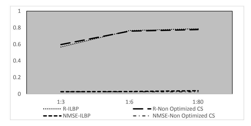
Figure 12 Performance comparison by NMSE and coefficient of correlation.
Subject to the coefficient of correlation, ILBP tends to perform better at a higher dielectric contrast. By qualitative observation, however, the elongation error appears more obvious at a higher dielectric contrast, which is also supported by the higher values of NMSE and NMAE as presented in Table 2. In general, ILBP can provide ECVT imaging but the elongation error was still observed for both low and high dielectric contrasts. This condition is not reliable enough for dynamic observations (moving object) or for medical tomography.
Based on quantitative measurement, Non-optimized CS performs better for higher dielectric contrast, which is supported by the smaller NMSE and the higher value of R in Table 2. However, Non-optimized CS fails to differentiate the imaging based on the dielectric contrast. This can be observed in Figure 6, Figure 8 and Figure 10. The three figures show the imaging of a static object at various dielectric contrasts with very similar visual appearance. In addition, overestimate imaging is another limitation of Non-optimized CS for ECVT imaging.
Based on quantitative measurement, ILBP and Non-optimized CS perform almost equally, as presented in Figure 12. The visual observation indicates that Non-optimized CS is able to reduce the elongation error that exists in ILBP. The imaging result tends to be more localized compared to ILBP. However, the imaging result of Non-optimized CS as presented in Figures 8 to Figure 10 still
overestimates the actual imaging as presented in Figure 4. In addition, some artifacts appear at the edge of the sensor.
It has been reported on CS framework modeling for MRI imaging that for image reconstruction with high undersampling measurement, CS image reconstruction employing a fixed or non-adaptive dictionary will typically suffer from many artifacts [19]. The ECVT imaging system mathematically has high undersampling measurement. Thus, the appearance of artifacts at the edge of the sensor boundary and the overestimate imaging are equitable. This issue is one of the challenges in developing a compressive-sensing framework for ECVT imaging that has a high undersampling projection (measurement) matrix. Moreover, the projection matrix for ECVT is structured instead of random, which can normally be optimized easily by a projection matrix optimization algorithm.
Apart from some limitations in the performance of Non-optimized CS for ECVT imaging, this method is promising for further development. Even though the resulting imaging still overestimates the actual image, the localized imaging is promising for medical tomography. Further development should be able to eliminate the overestimate result, which may distract analysis in real implementation. In addition, the imaging method based on compressive sensing is theoretically very well capable of providing imaging with less measurement data. This implies that an optimized CS for ECVT imaging will tend to reduce the number of required electrodes for providing acceptable ECVT imaging quality.
5.1 Analysis of Mutual Coherence Distribution (Gram Matrix)
The performance of CS on signal recovery or imaging can be indicated by the incoherency between the measurement (projection) matrix and the dictionary. The values of the off-diagonal components in the Gram matrix as explained in Definition 2 can be used to evaluate the performance of CS. Figure 11 presents the components of the off-diagonal elements of the Gram matrix for Nonoptimized CS. Theoretically, the higher the frequency of small values and the lower the frequency of high values (range 0-1), the more precise the recovery achieved by CS reconstruction. As presented in Figure 11, the frequency of high values for the off-diagonal components is still considerably high. Thus, the resulting imaging performance of Non-optimized CS is still not optimal. This indicates that the poor ECVT imaging quality by Non-optimized CS may be caused by an impropriate design of the measurement matrix or the dictionary. Since ECVT imaging has its own structured measurement matrix, another optimization approach is by designing an appropriate dictionary, which leads to an increase in the incoherency. As previously reported in [19], an adaptive
dictionary would be appropriate for such an ECVT imaging system with a very high undersampling measurement.
6 Conclusion and Future Work
A compressive sensing framework for signal recovery was elaborated. Mathematically, it is promising to be adopted for solving the ECVT imaging problem, which is an undetermined linear system. An early simulation of the CS framework for ECVT imaging was presented. The CS framework for ECVT imaging was implemented without optimization on the projection (measurement) matrix and dictionary, which is called Non-optimized compressive sensing.
A number of simulations were presented to evaluate the performance of Nonoptimized CS for ECVT imaging. ILBP, or Landweber algorithm, was used as the benchmark. Static object detection by using a cylindrical sensor with 8 electrodes was set up for the case study. The dielectric contrast was varied from low to high.
Based on the presented simulation, it cannot be said that ECVT imaging was successfully performed by Non-optimized CS. However, based on the early simulations, the proposed algorithm based on the CS framework is promising for use in ECVT imaging. Compared to ILBP, the proposed algorithm is able to reduce the existence of elongation error for various dielectric contrasts. However, the reconstructed ECVT image produced by Non-optimized CS still overestimates the actual imaging and produces some artifacts at the edge of the sensor, which may distract analysis in real implementation. The limitations of Non-optimized CS for ECVT imaging is theoretically equitable since the frequency of the high values for off-diagonal components of the Gram matrix is still considerably high. Moreover, for image reconstruction with high undersampling measurement, as in the case of ECVT imaging, the CS framework employing a fixed or non-adaptive dictionary will typically suffer from many artifacts [19].
The proposed ECVT imaging algorithm based on a non-optimized CS framework has a number of limitations, which have been theoretically clarified. However, it is promising for further development. The more localized imaging is one aspect of ECVT imaging by Non-optimized CS that is preferable compared to ILBP, especially for medical tomography purposes. Apart from that, the CS framework needs a smaller number of sampling data for signal recovery, which potentially implies a reduction of the number of required electrodes.
Based on previous research [19], it can be concluded that optimizing the projection matrix while maintaining a fixed dictionary for ECVT imaging, which is considered high-undersampling measurement, will not give significant improvement of the imaging quality. Optimization of the CS framework for ECVT imaging has to consider the dynamic dictionary framework. Another issue is that optimization should also consider the fact that the projection matrix of ECVT is structured instead of randomly assigned.
Acknowledgements
The authors would like to thank CTech Lab Edwar Technology for their supportive discussions and research resources and Tanri Abeng University for their support.