
1 Introduction
The development of micro-electromechanical system technology, digital electronics and wireless technology has led to the development of low-cost, low-power, tiny intelligent devices called sensors, with built-in sensing, computing and communication capabilities. Sensors are of limited capability, so a group of sensors is required to sense the area of interest. These collaborative efforts of sensors form a network, which is called a wireless sensor network (WSN). The typical work of a WSN is to monitor the area of interest and report to an observer system, called the base station (BS). Thus, every sensor senses its own area, processes the gathered data and transmits the processed data to the base station. Energy is consumed while sensing, processing and transmitting. Sensors are battery-powered and in most scenarios it is not feasible to replace or recharge the batteries. Therefore energy-efficiency is a major issue in the design of WSNs.
The deployment of sensors in WSNs is usually random, so it may happen that two of the sensors are in each other's vicinity. Consequently, their sensing data are more or less the same. Data aggregation can be used to eradicate these redundancies [1]. Sensors consume most of their energy while transmitting and receiving data. Clustering is a mechanism used to achieve energy efficiency and data aggregation in WSNs. In clustering, the network is partitioned into multiple subgroups of sensors; these subgroups are called clusters. Each cluster has a dedicated leader, called the cluster head (CH). The role of the CH is to collect the data from the cluster members, aggregate them and transmit them to the BS [2]. A CH can send the data directly to the BS or through intermediate CHs, depending on the architecture of the WSN. A comparative study of both approaches [3] has shown that the multi-hop approach is more energy efficient compared to the direct approach.
The main task of clustering protocols is the selection of efficient sensors as CHs and periodic rotation of the CHs to achieve uniform energy consumption. Low Energy Adaptive Clustered Hierarchy (LEACH) [4] was among the first algorithms developed to achieve energy efficiency by utilizing clustering. It employs randomized rotation of the CHs to distribute energy consumption all over the network. LEACH-Centralized, or LEACH-C [5], is a centralized version of LEACH in which the BS chooses the CH nodes using a simulated annealing approach from a set of nodes whose residual energy is more than the average node energy of the network. Multi-hop LEACH [3] eradicates the direct communication between the CHs and the BS by selecting an optimal path that adapts to multiple hops. The Hybrid Energy Efficient Distributed (HEED) protocol [6] uses the residual energy as a parameter when selecting the CHs.
Many of these protocols use the multi-hop communication model to reach the BS. As a result, the CHs nearer to the BS are loaded with intense relay traffic, which drains their energy faster. This leads to premature death of some nodes, causing network partition. This phenomenon is popularly known as the 'hot spot' or 'energy hole' problem [7]. In order to eradicate this problem several unequal clustering protocols have been proposed. In unequal clustering the CHs are assigned a different clustering range so that the network load can be distributed. The principle of unequality in clustering was first discussed by Soro and Heinzelman [8]. They proposed a scheme called Unequal Clustering Size (UCS). The main idea behind UCS is to form adaptive clusters based on their distance to the BS. Energy-efficient Unequal Clustering (EEUC) [9] is another unequal clustering mechanism, which selects CHs based on competition. Unequal Cluster-based Routing (UCR) [10] was one of the first protocols to solve the energy hole issue by using an unequal clustering approach. As in EEUC, in this approach the size of the cluster gradually decreases as one moves closer to the BS. Hierarchical Unequal Clustering Algorithm (HUCA) [11] is another unequal clustering approach, where the whole network is divided into horizontal grids and forms clusters in every grid.
However, there exist uncertainties within these approaches. Fuzzy logic is usually used to model human decision-making behavior and resolve uncertainties in decision-making. Gupta, et al. [12] proposed an algorithm for CH selection using fuzzy logic. In their approach, the BS calculates the CHs using three fuzzy descriptors: residual energy, node concentration, and centrality. The Cluster Head Election Mechanism using Fuzzy Logic (CHEF) [13] is an approach similar to that of Gupta, et al., but it employs a distributed approach using fuzzy logic for CH selection. Similarly, Mao, et al. [14] use fuzzy logic to calculate a chance value and the range of the tentative CHs. In the Fuzzy Energy-Aware Unequal Clustering algorithm (EAUCF) [15], the authors address the hot spot problem by unequal clustering using fuzzy logic. The Low-Energy Adaptive Unequal Clustering Protocol using Fuzzy C-Means (LAUCF) [16] is an unequal cluster based approach that utilizes the fuzzy c-means algorithm to form disjoint clusters of different sizes.
In a randomly deployed WSN, node density plays a major role; however, the clustering approaches proposed so far do not properly tackle this issue. Therefore, in this paper, a fuzzy logic based unequal clustering approach is proposed to resolve the stated problem of unequal energy drainage. Another fuzzy based approach is used to decide the clustering range of the CHs. Moreover, a multi-hop based routing approach is used, in which a weight function is utilized to optimize the selection of relay nodes. The most notable features of the proposed methodology can be summarized as follows:
- 1. The CHs are selected non-probabilistically: the nodes wait for a certain amount of time before declaring themselves a CH. The waiting time is inversely proportional to fitness (chance).
- 2. Chance is calculated using fuzzy logic: the Chance value is a blend of three input parameters (residual energy, centrality and density) subjected to a fuzzy inference system (FIS) to get the value.
- 3. The CHs have different clustering ranges: the clustering range is a function of node chance and distance to BS, which is calculated using another FIS.
- 4. Multi-hop mode of data communication: a cost function based on node chance and distance to BS is used to select the CHs most suitable for the relaying of data packets.
The remainder of this paper is organized as follows. In Section 2, the system model of our proposed methodology is discussed. Section 3 briefly elaborates the problem statement. The proposed methodology is described in Section 4. In Section 5, a detailed analysis of the proposed approach is given. Section 6
presents a extensive simulation and the results of the proposed work. Finally, the conclusion is given in Section 7.
2 System Preliminaries
This paper considers a sensor network consisting of n sensor nodes randomly deployed over an area. The sensors continuously sense the area and send the sensed data to a BS through intermediate sensors. Each sensor node can operate either as a cluster member to sense the environment and send the data to a CH or as a CH to collect data, compress them and send them to the BS. Apart from this functionality, a CH can also work as a relay node. The sensors and the BS are stationary after deployment. All the sensors are homogeneous and have the exact same amount of initial energy. The sensors are left unattended after deployment and therefore battery recharge is not feasible. Each sensor is uniquely identified by an identifier (ID). The sensors have the ability to vary the amount of transmission power depending on the distance of the receiving node. The distance between the sensors can be calculated on the basis of received signal strength (RSS) if the transmitting power is known. The radio links are symmetric. Thus, the communication between any two nodes requires the same transmission power.
However, in a real-world scenario some of the assumptions made about the system model do not hold. For example, it is assumed that the distance between any pair of sensors can be calculated based on RSS but because of multi-path fading and the shadowing effect, the measured distance is subject to error. Still, RSS can give a good approximation of the distance with a low energy overhead [17].
In this work, the first-order radio model is applied as described in [18] to model the energy dissipation. If the distance between the receiver and the transmitter is lower than a threshold value \(d_0\), the free space model (\(d^2\) power loss) is used. Otherwise the multipath fading channel model (\(d^4\) power loss) is used. The energy required to transmit an l-bit packet over distance d is expressed in Eq. (1):
\[E_{Tx}(l,d) = lE_{Elec} + l\varepsilon d^{\alpha} = \begin{cases} lE_{Elec} + l\varepsilon_{fs}d^{2}, d < d_{0} \\ lE_{Elec} + l\varepsilon_{mp}d^{4}, d \ge d_{0} \end{cases}\](1)
where \(E_{Elec}\) energy is required to run the transceiver, which depends on factors such as digital coding and modulation, and \(\varepsilon_{fs}d^2\) or \(\varepsilon_{mn}d^4\) is the amplifier
energy, which depends on the transmission distance and an acceptable bit error rate. The threshold value 0 d can be obtained from Eq. (2),
\[d_0 = \sqrt{\varepsilon_{fs}/\varepsilon_{mp}} \tag{2}\]
The amount of radio energy that dissipates when receiving a message is given by Eq. (3),
\[E_{Rx}(l) = lE_{Elec} \tag{3}\]
We assume that the sensed information is highly correlated, therefore the CH aggregates the data gathered from the member nodes and compresses it into a single packet. In the proposed methodology, we assume that ( / / ) E nJ bit signal DA of energy is consumed by the CH for data aggregation.
3 Problem Statement
Let's assume all of the abovementioned assumptions hold and n sensor nodes are deployed. Considering energy saving, the goal of a good clustering algorithm is to identify a set of CHs that covers the entire area. Each node i S , where1≤ ≤i n , must be mapped to exactly one CH from the set of CHs. Let Li be the lifetime of node i S . The lifetime of the network is then defined as follows [19]:
- 1. first node dies (FND): FND = min (L1L2L3… Ln)
- 2. half of nodes alive (HNA): HNA = median (L1L2L3… Ln)
- 3. last node dies (LND): LND = max (L1L2L3… Ln)
The purpose of a good clustering algorithm is to be able to maximize the above three metrics. The existing clustering algorithms usually consider a uniform distribution of nodes throughout the WSN, whereas in most practical applications the nodes are deployed randomly. Hence, if the underlying clustering algorithm does not consider the node distribution, it can lead to an unbalanced topological structure and some nodes die rapidly, causing partitioning of the network. Some algorithms (such as LEACH, HEED, etc.) divide the network into nearly equally sized clusters and the CH communicates with the BS directly. Some use multi-hop communication. In the former case, the more distant nodes die rapidly and in the latter case the nodes closer to the BS die quickly. Some algorithms use inequality in clustering to balance energy consumption, which has proved to be more proficient than equality. Hence, based on the above observations, the algorithm proposed in this paper tries to construct a more balanced clustering scheme based on inequality in order to extend the lifetime of the network.
4 Proposed Methodology
In this section, the proposed methodology is discussed. The proposed method works in rounds. For each round the proposed approach consists of three stages: the CH selection phase, the cluster set-up phase and the steady-state phase. The neighborhood discovery phase is executed only once, before the start of the first round. In this study, a fuzzy inference system (FIS) was used to handle ambiguity. An FIS is a system that uses fuzzy set theory to map an input space to an output space. Here, the Mamdani method of fuzzy inference technique [20] was used.
4.1 Neighborhood Discovery Phase
The algorithm starts with the neighborhood discovery phase, in which the BS broadcasts a 'hello' message. Upon receiving this message, a node calculates its distance from the BS. The receiving node of the 'hello' message broadcasts a 'hello reply' message (\(hello\_r\_msg\)) containing the sender id within the range \(R_{\max}\), where \(R_{\max}\) is the maximum clustering range which is broadcast by the BS in the 'hello' message. The receiving node of \(hello\_r\_msg\) adds the sender as its neighbor, calculates the distance to the neighbor and records the sender id along with its distance. Whenever any node has residual energy below a given threshold, it will broadcast itself as dead by sending a 'dead' message (\(dead\_msg\)), upon which the receiving nodes of the \(dead\_msg\) update their neighborhood information. The neighborhood discovery phase is carried out only once during the time of network deployment.
4.2 Cluster Head Selection Phase
At the end of the neighborhood discovery phase, each node waits for WaitTime before broadcasting a Candidate CH Message (can_msg). WaitTime is calculated as follows:
\[WaitTime = \frac{1}{Chance} \tag{4}\] where Chance is the output of the FIS. The value of the Chance variable ranges between 0 and 1, so the higher the value the shorter the waiting time. A higher value means the node is more suitable as a CH.
The input variables for FIS are residual energy, centrality and node density. These variables are defined as follows:
- 1. Residual energy remaining energy level of anode
- 2. Centrality a value that classifies the nodes based on how central they are to a cluster
3. Node density – number of nodes present in clustering range Ri
Ri denotes the clustering range of node i. In the initial round, the value of Ri is set to Rmax . From the second round onward the clustering range is further adjusted using another FIS. The clustering range adjustment is described in the follow-up section after the description of the chance value.
A fuzzy set that illustrates the residual energy input variable for the FIS is represented in Figure 1(a). The linguistic variables for this fuzzy set are low, mid and high. A triangular membership function is used for mid and a trapezoidal membership function is used for the linguistic variables low and high.
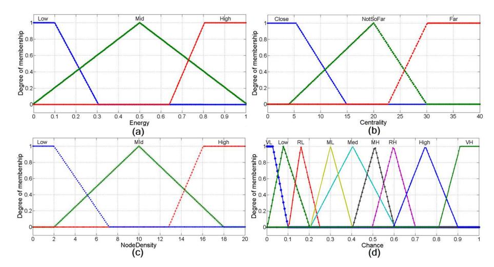
Figure 1 (a) Fuzzy set for input variable Residual Energy. (b) Fuzzy set for input variable Centrality. (c) Fuzzy set for input variable Node Density. (d) Fuzzy set for output variable Chance.
The second fuzzy set contains the centrality of the candidate CHs. A fuzzy set that illustrates the input variable Centrality for the FIS is shown in Figure 1(b). The linguistic variables for this fuzzy set are close, not so far and far. A triangular membership function is used for not so far and a trapezoidal membership function is used for the linguistic variables close and far.
The third fuzzy set contains the node density of the candidate CHs. A fuzzy set that illustrates the input variable Node Density for the FIS is represented in Figure 1(c). The linguistic variables for this fuzzy set are low, mid and high. A triangular membership function is used for mid and a trapezoidal membership function is used for the linguistic variables low and high.
The only fuzzy output variable is the Chance value of the candidate CHs. A fuzzy set that illustrates Chance is illustrated in Figure 1(d). There are nine linguistic variables used for this fuzzy set, i.e. very low, low, rather low, med low, medium, med high, rather high, high and very high. The very low and very high variables have a trapezoidal membership function and the remaining seven linguistic variables are represented by triangular membership functions.
The calculation of the Chance variable is accomplished by using predefined fuzzy if-then mapping rules to resolve the uncertainties. There are 27 fuzzy mapping rules, as listed in Table 1. By applying these fuzzy if-then mapping rules on the inputs, the fuzzy output variable Chance is generated.
| Table 1 | Fuzzy mapping rule base of first FIS. |
|---|
| SI no. | Residual energy | Centrality | Node density | Chance |
|---|---|---|---|---|
| 1 | Low | Close | Low | Rather Low(RL) |
| 2 | Low | Close | Med | Medium Low(ML) |
| 3 | Low | Close | High | Rather Low(RL) |
| 4 | Low | NSF | Low | Low |
| 5 | Low | NSF | Med | Rather Low(RL) |
| 6 | Low | NSF | High | Low |
| 7 | Low | Far | Low | Very Low(VL) |
| 8 | Low | Far | Med | Low |
| 9 | Low | Far | High | Very Low(VL) |
| 10 | Med | Close | Low | Medium |
| 11 | Med | Close | Med | Medium High(MH) |
| 12 | Med | Close | High | Medium |
| 13 | Med | NSF | Low | Medium Low(ML) |
| 14 | Med | NSF | Med | Medium |
| 15 | Med | NSF | High | Medium Low(ML) |
| 16 | Med | Far | Low | Rather Low(RL) |
| 17 | Med | Far | Med | Medium Low(ML) |
| 18 | Med | Far | High | Rather Low(RL) |
| 19 | High | Close | Low | High |
| 20 | High | Close | Med | Very High(VH) |
| 21 | High | Close | High | High |
| 22 | High | NSF | Low | Rather High(RH) |
| 23 | High | NSF | Med | High |
| 24 | High | NSF | High | Rather High(RH) |
| 25 | High | Far | Low | Medium High(MH) |
| 26 | High | Far | Med | Rather High(RH) |
| 27 | High | Far | High | Medium High(MH) |
The output fuzzy variable has to be defuzzified to a single crisp value so that it can be used in practice. In this study, the center of gravity method [21] was used for defuzzyfication. The value is given by Eq. (5):
\[Chance = \frac{\sum_{i=1}^{n} U_i * a_i}{\sum_{i=1}^{n} U_i}\] (5)
where \(U_i\) is the output of the rule base and \(a_i\) is the center of the output membership function.
When the waiting time is over, the candidate CHs broadcast a can_msg within their clustering range. The can_msg consists of the node id and the Chance value. At this time, the clustering range of the candidate CHs is further adjusted using another FIS. The input variables for FIS for the clustering range are the distance to the BS and the Chance value of the node. The parameter Distance to BS signifies the node's distance from the BS and Chance is the outcome of the first FIS.
An input fuzzy set that illustrates the Chance variable for the second FIS is represented in Figure 2(a). The linguistic variables for this fuzzy set are low, mid and high. A triangular membership function is used for mid and a trapezoidal membership function is used for the linguistic variables low and high.
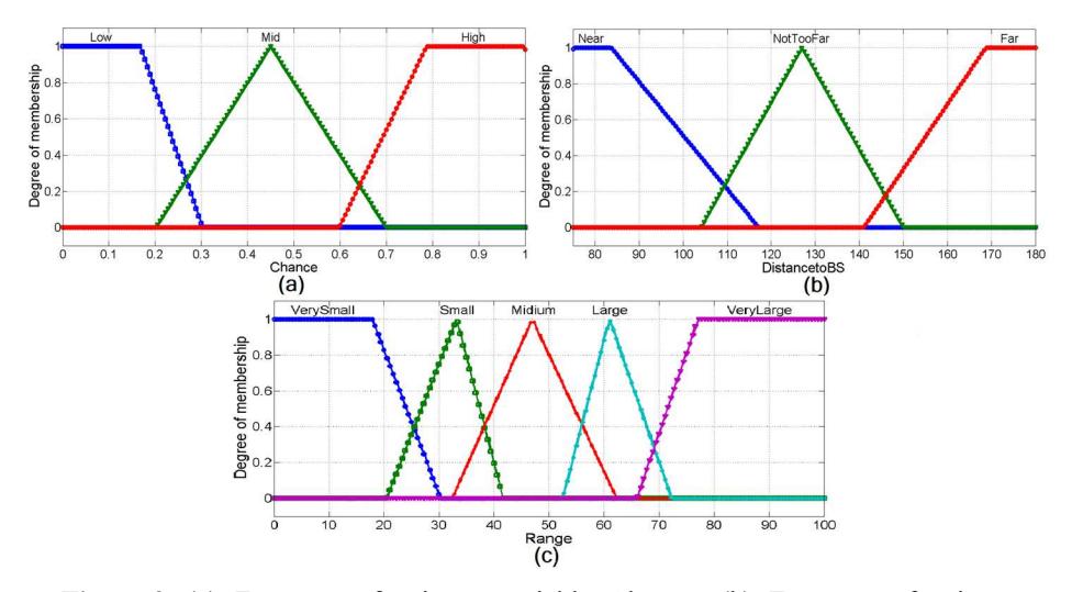
Figure 2 (a) Fuzzy set for input variable Chance. (b) Fuzzy set for input variable Distance to BS. (c) Fuzzy set for output variable Range.
An input fuzzy set that illustrates the Distance to BS variable for the second FIS is represented in Figure 2(b). The linguistic variables for this fuzzy set are near, not too far and far. A triangular membership function is used for not too far and a trapezoidal membership function is used for the linguistic variables near and far.
| SI no. | Chance | Distance to BS | Range |
|---|---|---|---|
| 1 | Low | Near | Very Small |
| 2 | Low | Not too far | Small |
| 3 | Low | Far | Medium |
| 4 | Med | Near | Small |
| 5 | Med | Not too far | Medium |
| 6 | Med | Far | Large |
| 7 | High | Near | Medium |
| 8 | High | Not too far | Large |
| 9 | High | Far | Very Large |
Table 2 Fuzzy mapping rule base of second FIS.
The only fuzzy output variable of the second FIS is Range. A fuzzy set that illustrates this variable is represented in Figure 2(c). There are five linguistic variables used for this fuzzy set, i.e. very small, small, medium, large and very large. The very small and very large variables have a trapezoidal membership function and the remaining five linguistic variables are represented by triangular membership functions. In this work, mostly triangular membership functions were used because of their simplicity and because they require less computation compared to other membership functions.
The calculation of Range is accomplished by using predefined fuzzy if-then mapping rules, as listed in Table 2. There are 9 rules, based on the two fuzzy inputs. By applying these fuzzy if-then mapping rules on the inputs, the fuzzy output variable Range is generated. Defuzzyfication is accomplished by Eq. (5), as specified above.
The candidate CHs are the nodes that have sent a can_msg. After that either they did not receive any can_msg or their Chance value is higher than that of their neighbors. When a node has a lower Chance value it cancels its timer and decides to become a cluster member. It can also occur that a node with a lower Chance value sends a can_msg, in which case the node quits the election process and becomes a cluster member. This competition guarantees that only the node with the highest Chance value will become CH and there will be no other CHs within its competition range. It also makes sure that there no region inside the network is overlooked.
4.3 Cluster set-up Phase
In this phase, the remaining candidate CHs send a CH message (CH_msg) within the range of TH-BS. The CH_msg consists of node id, Chance and
Distance to BS. Upon receiving a CH_msg, the CH maintains a table of its neighbor CHs. The entries in that table are: neighbor CH node id, Chance and Distance to BS. Upon receiving multiple CH messages, non-CH nodes will join the closest CH by sending a member message (mem_msg). Then each CH prepares a TDMA schedule telling each member node when to transmit the message for which it received a mem_msg. This TDMA schedule is broadcast back to the member nodes of the cluster.
4.4 Steady-state Phase
In this phase, the actual data transmission begins after the CHs have been selected and the TDMA schedule has been prepared. Every non-CH node sends its data according to the predefined TDMA schedule and then goes into sleep state. The CH nodes must keep their receiver on to be able to receive data from the non-CH nodes in their cluster.
4.5 Inter-cluster Multi-hop Routing
After receiving all the data from the non-CH nodes, the CH aggregates the data, compresses them and passes them to the BS. In this work, an inter-cluster multi-hop based routing approach was employed. Threshold value TH-BS is used by the CHs to determine whether to send the data to the next CH or to the BS directly. For instance, if CH<sub>i</sub> has a packet to send and its distance to the BS is smaller than TH-BS, it will send the packet directly to the BS. Otherwise CH<sub>i</sub> will choose a relay CH from its neighboring clusters (if any exist). The value of TH-BS is quite small compared to the maximum transmission range because long-distance communication requires more energy compared to multiple short-distance communications. Moreover, channel interference increases with an increase in communication distance [22].
Suppose \(CH_i\) chooses \(CH_j\) as its relay node. For simplicity, it is assumed that the free space propagation model is used and \(CH_j\) can communicate directly with the BS. To deliver an l-bit message to the BS, the amount of energy consumed by \(CH_i\) and \(CH_j\) can be calculated with Eq. (6):
\[\begin{split} E_{\text{Relay}} &= E_{Tx} \Big( l, d(CH_i, CH_j) \Big) + E_{Rx} \Big( l \Big) + E_{Tx} \Big( l, d(CH_j, BS) \Big) \\ &= l(E_{Elec} + \varepsilon_{fs} d^2 (CH_i, CH_j)) + lE_{Elec} + l(E_{Elec} + \varepsilon_{fs} d^2 (CH_j, BS)) \\ &= 3lE_{Elec} + l\varepsilon_{fs} (d^2 (CH_i, CH_j) + d^2 (CH_j, BS)) \end{split} \tag{6}\]
It is obvious that \(d^2(CH_i, CH_j) + d^2(CH_j, BS)\) has the largest share in the total energy consumed during data forwarding. This indicates that the larger the distance, the more energy is required to transmit data. Furthermore, CHs with a higher Chance value are likely to have a greater potential to become a relay node. Thus, we propose a cost function that takes into account the above two factors for selecting the appropriate relay node. This is calculated with Eq. (7), as follows:
\[CH_{j}.Cost = \rho \frac{\sum Chance(CH_{i})}{CH_{i}.Chance} + (1 - \rho) \frac{d^{2}(CH_{i}, CH_{j}) + d^{2}(CH_{j}, BS)}{d^{2}(CH_{i}, BS)}\](7)
where \(\sum Chance(CH_i)\) is the sum of the Chance values of the neighboring CHs of \(CH_i\), and \(CH_j\). Chance is the Chance value of \(CH_j\) and \(\rho\) is the weighing factor. The value of \(\rho\) is between 0 and 1. After getting the cost of every neighbor CH, the CH will choose the minimum-cost neighbor CH as its relay CH. This is given as in Eq. (9):
\[CH_{Relay} = \left\{ CH_j \middle| CH_j.C \text{ os } t \text{ is } \min imum \right\}\] (8)
5 Protocol Analysis
Energy consumption per round roughly happens in two distinct phases: the cluster set-up phase and the data transfer phase. As outlined in Section 4, each round consists of selecting a set of CHs chosen from m candidate CHs. Each candidate CH sends a \(can\_msg\) within the range \(R_i\). The energy consumed by these candidate CHs per round is given by Eq. (9):
\[E_{Can\_msg} = ml(E_{Elec} + l\varepsilon_{fs}R_i^2) + \frac{h\pi R_i^2}{A^2}lE_{Elec}\] (9)
The first term in Eq. (9) represents the energy consumed by the candidate CHs in transmitting \(can\_msg\). The second term signifies the energy consumed in receiving the \(can\_msg\) from the other candidate CHs. The number of messages received is based on the estimate that h candidate CHs will fall within one cluster range, where \(A^2\) is the area of the network. Similarly, Eq. (10) represents the energy consumed by the selected CH to transmit the \(CH\_msg\) and Eq. (11) represents the energy consumed by the non-CH nodes in sending the \(mem\_msg\), where n represents the number of nodes and k represents the number of CHs.
\[E_{CH\_msg} = kl(E_{Elec} + l\varepsilon_{fs}R_i^2) + kl\left(\frac{n\pi R_i^2}{A^2}\right)E_{Elec}\] (10)
\[E_{mem\_msg} = (n - k)(E_{Elec} + l\varepsilon_{fs}d^{2}) + \left(\frac{k\pi R_{i}^{2}}{A^{2}}\right)lE_{Elec}\] (11)
The energy consumed in sending the schedule message is equivalent to Eq. (10). Hence, the total energy consumed during the clustering phase is given by Eq. (12):
\[E_{Cluster \ set \ up} = E_{Can \ msg} + 2E_{CH \ msg} + E_{mem \ msg}\] (12)
In the data transmission phase, each member node sends a packet to its CH. This is given by Eq. (13):
\[E_{Member\_data} = l(n-k)(E_{Elec} + l\varepsilon_{fs}d^{2})\] (13)
Then every CH sends the aggregated messages to the BS through a relay CH. This is given by Eq. (14):
\[E_{CH\_data} = lk(E_{Elec} + l\varepsilon_{fs}d^2) + \left(\frac{k\pi R_{TH\_BS}^2}{A^2}\right) lk(E_{Elec} + E_{DA})\] (14)
Theorem 1. There is at most one CH in the cluster range of any CH
Proof. As mentioned above, Eq. (5) ensures that different nodes have different waiting times. Let us assume that node \(n_i\) has a shorter waiting time and sent a \(can\_msg\) in its cluster range \(R_i\). Consequently, the nodes within the cluster range with a longer waiting time will cancel their timer and become a cluster member. It is also possible that a node with a lower Chance value has sent a \(can\_msg\), in such case the node will quit the election. Therefore, it is ensured that only the node with the highest chance value will be the CH and there will be no other CHs within its competition range.
Theorem 2. The cluster head set generated by the proposed approach covers all nodes
Proof. According to Theorem 1, there is no more than one CH within the cluster range of any CH. When the cluster head selection phase is over, each node in the network either is the CH or a member node of the cluster. Let us assume that there is a node that cannot join any cluster, which means the node is not able to receive a can_msg. In that case, when the waiting time is over, the node broadcasts a can_msg in its clustering range and since there is no candidate CH within its clustering range, it will declare itself the CH by sending a CH msg.
Theorem 3. The control message complexity of the network is O(N) and the processing time complexity is O(1)
Proof. Initially every node sends a hello_r_msg and when any node has residual energy below a given threshold it will send a dead_msg. As these messages occur once in a network's lifetime, we can neglect these messages.
Every round, m nodes send a can_msg ( m < n ). k nodes send a CH_msg, k scheduled messages, and n k − non-CH nodes send a mem_msg. Hence, the overall complexity of the network is (n k m k k n m k − + + + = + + ) . Therefore, the overall complexity of the control messages in the network is O n( ). The clustering process of the proposed approach is distributed. Thus, the time complexity of the entire network is equivalent to the time complexity of a single node, i.e. O(1) . In other words, the time complexity of the network is a constant and has nothing to do with the size of the network.
6 Simulation and Result Discussion
In this section, the results of a simulation experiment are presented to illustrate the effectiveness of the proposed method. For simplicity an ideal MAC layer and an error-free communication link were used. Energy was consumed whenever a sensor sent data, received data and performed data aggregation. The proposed algorithm was compared with LEACH, UCR and EAUCF.
The metrics for comparing the algorithms were: the lifetime of the network in terms of rounds, FND, HNA, LND, the average number of clusters per round until FND, the average number of clusters per round from FND until HNA, the average number of clusters per round from HNA until LND, and the packet delivery ratio (PDR). The FND and HNA metrics are quite powerful compared to LND because when half of the nodes are dead, the network is of almost no use. PDR is defined as the ratio between the total number of packets received at the BS and the total number of packets generated in the network.
The sensor nodes were randomly deployed over a 100 m x 100 m area. There was only one BS, located at (50 m, 175 m) for Scenario I and at (50 m, 50 m) for Scenario II. The rest of the parameters were the same for both scenarios. The details of the parameters and their values are given in Table 3. All the results in the scenarios were plotted by taking the mean value over 20 experiments. For determining the parameter settings, we used Scenario I. The aggregation ratio for the simulation was set to 10% and the same mechanism was used as described in [15]. Unless otherwise specified, Rmax was set to 80 m, ρ to 0.4 and TH-BS to 60 m. These values were found appropriate by running the simulation described below.
| Parameter | Values |
|---|---|
| Network dimension | (0,0)-(100,100) |
| Base station location | (50,175)(50,50) |
| Nodes | 100 |
| Initial energy | 1 J |
| fs ε | 10 pJ/bit/m2 |
| mp ε | 0.0013 pJ/bit/m4 |
| EElec | 50 nJ/bit |
| d 0 | 87m |
| EDA | 5 nJ/bit/signal |
| Data packet size | 4000bits |
Table 3 Simulation parameters.
6.1 Parameter Settings
There are three main parameters in the proposed method that influence the clustering and data forwarding, namely Rmax , ρ and TH-BS. The value of Rmax was set to 80 m as given by [10], which was found suitable for the proposed method. First, the effect of TH-BS on the lifetime of the network was examined. The impact of TH-BS on the lifetime of the network for different TH-BS values was observed; the result is shown in Figure 3(a). The values of the network were set as described above and the value of TH-BS was varied from 30 m to 80 m. The highest lifetime was achieved when the value of TH-BS was 60 m. This confirms our problem statement, i.e. if TH-BS is too large, more energy is consumed and, in contrast, if TH-BS is too small, the same data will be received and sent multiple times, which requires more energy.
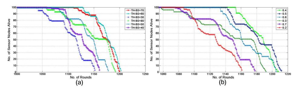
Figure 3 (a) Network lifetime with different values for TH-BS. (b) Network lifetime for different values of ρ .
Secondly, the impact of ρ on the lifetime of the network was studied. As described above, distance is an important factor in the total energy consumed during the forwarding of data; at the same time the Chance value of the relaying node cannot be ignored. Hence, ρ is the weighing factor, which decides how much weight needs to be given to each parameter. Basically, we need a value of ρ that will increase the lifetime expectancy of the network. The network was checked for different values of ρ , from 0.2 to 0.7. The highest lifetime was achieved when the value of ρ was set to 0.4. The result of the simulation is shown in Figure 3(b).
6.2 Comparison: Scenario I
In this part, the proposed method is compared with the LEACH, UCR, and EAUCF algorithms. In Scenario I, the BS is positioned at (50 m, 175 m). The aim here was to observe the behavior of the network when the BS is placed outside the network.
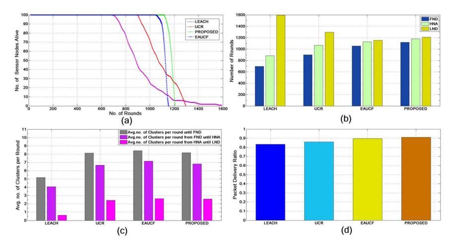
Figure 4 Scenario I. (a) Distribution of the live node per round. (b) Lifetime metrics FND, HNA and LND. (c) Average number of clusters per round. (d) Packet delivery ratio.
The value of ρ was set to 0.4 and TH-BS to 60 m for the proposed method. The maximum clustering range was set to 65 m for UCR, as we found it the most promising for our configuration. The other three algorithms, except LEACH, send their data packets to the BS using multi-hop routing. First, the lifetime of all four approaches was compared. Figure 4(a) demonstrates the distribution of the live nodes with respect to the number of rounds until LND. It is evident from the figure that the proposed method was more stable compared to the others because the death of the sensor nodes begins later and continues linearly.
The second comparison was made on the basis of the FND, HNA and LND metrics. Figure 4(b) shows a detailed comparison of the three metrics for all four approaches. As stated above, FND and HNA are the two most important factors considering the lifetime of the network. The performances with respect to the FND metric of the proposed approach and EAUCF were close to each other, but the proposed approach was 56.3% more efficient than LEACH, 23.1% more efficient than UCR, and 8.6% more efficient than EAUCF. Similarly, the proposed approach with respect to the HNA metric was 33.6% more efficient than LEACH, 10.5% more efficient than UCR and 4.7% more efficient than EAUCF. The performance of LEACH was the poorest compared to the other three, because it uses a purely probabilistic approach to clustering and data are transmitted directly from the CHs to the BS. UCR showed an improvement over LEACH as it gives a different clustering range to the CHs and uses multi-hop routing to forward the data packets. However, it is clearly visible from the figure that the fuzzy based unequal clustering approach showed better performance compared to LEACH and UCR. This is due to the fact that the fuzzy unequal clustering approach resolves uncertainties in assigning a clustering range to a CH, depending on multiple inputs in contrast to only distance in UCR. However, for three reasons, the proposed method showed a considerable improvement over EAUCF. Firstly, it employs a fuzzy logic based CH selection approach in contrast to the probabilistic CH selection in EAUCF. Secondly, it considers the chance value to ascertain node fitness along with distance to the BS when assigning the clustering range. Thirdly, it achieves an efficient selection of relay nodes.
The third comparison was based on the average number of clusters per round until FND, the average number of clusters per round from FND until HNA, and the average number of clusters per round from HNA until LND. As shown in Figure 4(c), the proposed algorithm had good results for all three metrics. If the number of CHs is smaller, then the number of nodes per cluster increases. Consequently, the energy consumption of the CHs will increase. On the other hand, if it is too large then a lot of energy will be wasted in cluster formation. Therefore, we need to have the right number of CHs per round to push the lifetime of the overall network. The number of CHs in the case of LEACH is smaller, because in LEACH a certain percentage of nodes are selected probabilistically as CHs. However, the other three approaches, including the proposed approach, use unequal clustering, which creates smaller clusters around the BS. As a result, there are large numbers of CHs until FND and the number decreases towards HNA and is reduced further until LND. However, compared to EAUCF, the proposed approach has a slightly lower percentage of CHs per round.
The fourth comparison was made on the basis of the packet delivery ratio (PDR). Figure 4(d) represents the ratio of the number of packets generated in the network to the number of packets that reached the BS. It can be observed from the figure that the proposed approach had the highest ratio (91.17%). It also turned out to be 8.84% more efficient than LEACH, 5.93% more efficient than UCR and 1.56% more efficient than EAUCF.
6.3 Comparison: Scenario II
In this scenario, the BS was located at the center of the network i.e. at (50 m, 50 m). The aim of this scenario was to observe the behavior of the network when the BS is placed outside the network.
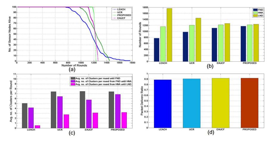
Figure 5 Scenario II. (a) Distribution of live nodes per round. (b) Lifetime metrics FND, HNA and LND. (c) Average number of clusters per round. (d) Packet delivery ratio.
For this scenario the same configuration was used as listed in Table 3 with a slight modification of some of the parameters. As the BS is at the center, a different value of Rmax and TH-BS is needed. Hence, Rmax was set to 40 m and TH-BS to 30 m.
The first comparison is based on the lifetime of the network. Figure 5(a) demonstrates the distribution of the live nodes with respect to the number of rounds for each method. It shows significant improvement in lifetime compared to Scenario I. This result is quite obvious because when we put the BS at the center of the network two things happen: first, less energy is required to communicate with the BS, and secondly, there are more CHs that can communicate to the BS directly. Again, the performance of the proposed method was well ahead of the other three for the same reason as described under Scenario I.
The second comparison is based on the FND, HNA and LND metrics. Figure 5(b) shows a detailed comparison of the three metrics for all four approaches. Compared to Scenario I, the values of the FND, HNA and LND metrics increased because of the location factor of the BS. However, similar to the previous scenario, the proposed approach outperformed the other three. The proposed approach was 51.3% more efficient than LEACH, 20.0% more efficient than UCR, and 7.9% more efficient than the EAUCF with regards to the FND metric. Similarly, the proposed approach was 10.2% more efficient than LEACH with regards to the HNA metric. The performance of LEACH was also the poorest in this scenario. It is clearly visible from the figure that the unequal clustering approach shows better performance compared to LEACH, which strongly supports the use of unequal clustering in WSNs. However, the proposed method shows quite an improvement over UCR and EAUCF with regards to the FND for the same reason as mentioned with regards to Scenario I.
Figure 5(c) displays the average number of clusters per round for each method. Compared to Scenario I, the average number of CHs in all of the approaches was smaller; this is because of the location of the BS. In the case of LEACH, the difference is quite significant; this is because of the extended lifetime of this approach from the moment when the first node dies and the fact that it generates a constant number of clusters until the first node dies, after which it keeps reducing as more nodes die. The other three approaches maintain a good number of CHs. However, compared to EAUCF, the proposed approach has a slightly lower percentage of CHs per round.
The fourth comparison is based on the packet delivery ratio (PDR). Figure 5(d) represents the ratio between the number of packets generated in the network and the number of packets that reached the BS. Similar to Scenario I, here also the proposed approach had the highest PDR ratio (92.43%). It also turned out to be 3.93% more efficient than LEACH, 1.98% more efficient than UCR, and 0.87% more efficient than EAUCF in this scenario.
So by comparing Scenario I with Scenario II, it can be stated that when the BS is moved further away from the center of the network, the improvement in performance between the proposed approach and the other three algorithms increases significantly.
7 Conclusion
In this paper, an unequal clustering algorithm using fuzzy logic with distributed self-organization for WSNs of non-uniform distribution was proposed. The main objective of this method was to push the boundaries of the lifetime of the WSN by means of an even distribution of the workload. To achieve this goal, the main focus was on selecting the most efficient node as CH and then assigning the clustering range that is most suitable regarding fitness and location. Thus, the proposed method creates an optimal configuration of the clusters and the relay node selection creates a stable route.
The algorithm was examined by conducting an extensive simulation. According to the results, the proposed method has a better performance compared to existing clustering approaches. It was shown that the proposed method is feasible and improves the network's lifetime significantly. The proposed method works for WSNs with stationary homogeneous nodes. In future work, we can extend our approach to heterogeneous networks with mobility support.