1 Introduction

Geo-demographic analysis (GDA) is a tool to discover hidden patterns in geodemographic data when studying the characteristics of a population based on geographical area [1-4]. GDA is often used with a clustering technique to identify groups or clusters in the geo-demographic data based on two main assumptions: people living in the same location usually have similar characteristics, and areas can be grouped according to their population [1]. Fuzzy clustering is often used because of its ability to reduce ecological fallacy issues and to generate a specific distribution of a population's characteristics [5,6]. Using fuzzy clustering, an object has membership values and can be categorized into one or more clusters based on its probability in every cluster [7].

A clustering algorithm that is effective for GDA is the fuzzy geographically weighted clustering (FGWC) algorithm. This is an improvement of the Fuzzy C-Means (FCM) algorithm using geographical effect in the membership value calculation [5]. FGWC has a weakness in the initialization process, i.e. it determines cluster centers randomly, which can lead to a local optimum. Because the global optimum solution may not be reached, FGWC does not ensure reaching better clustering quality. This weakness has been overcome by integrating a metaheuristic algorithm – ant colony optimization (ACO) – resulting in the FGWC-ACO algorithm [8]. However, the addition of ACO to FGWC leads to another weakness. The FGWC-ACO algorithm runs slower than the FGWC algorithm because when running ACO there are repeated iterations to find the best solution, i.e. the global optimum for the objective function.

Several researches have proved that context-based clustering can increase the running time of clustering algorithms [2,9,10]. Context-based clustering is a technique of dividing data into groups based on a defined context variable without reducing clustering quality [9]. Context-based clustering by applying auxiliary variables in FCM has been introduced in [11]. It also has been implemented in the standard FGWC algorithm [10]. In the FGWC-ACO algorithm, context-based clustering is implemented, resulting in the CFGWC-ACO algorithm [12]. These researches showed that the proposed algorithm using context-based clustering is faster than the original algorithm. The researches also proved that implementation of context variables not only decreases the running time but also increases clustering quality by focusing the cluster centers on a specific purpose.

Parallel programming is another way of increasing computation performance without reducing accuracy. One way to utilize CPU performance in parallel computing is programming by using graphical processing units (GPUs). GPUs with many cores can run thousands of threads in parallel [13]. Compute Unified Device Architecture (CUDA) is a platform model of parallel programming designed by NVIDIA. CUDA can improve computation performance by utilizing the abilities of GPUs. Some researchers have proved that CUDA is able to increase the running time of clustering algorithms, such as Jiang et al., who have reported that CUDA implementation can increase the running time of the harmony K-means algorithm successfully, especially if the cluster number is large [14]. Another research, by Glenis and Pham, successfully proved performance acceleration of FCM by implementing CUDA [15].

The present research was aimed at improving the performance of the FGWC-ACO algorithm and context-based clustering in FGWC-ACO (CFGWC-ACO) by using CUDA parallel programming. Implementation was done using two parallel strategies: 1) in the stage of solution evaluation (FGWC-ACO-CUDA-1), and 2) in the stage of both solution construction and solution evaluation (FGWC-ACO-CUDA-2). The proposed method classifies processes of the algorithm that can be run in parallel and then puts each of them into GPU threads. The strategy is to implement CUDA parallel programming in the original algorithms in order to get significant computation acceleration without reducing clustering quality.

The rest of this paper is organized as follows. Section 2 explains the theoretical background of this research. Section 3 gives the method that is proposed to resolve the weakness of the original algorithm. Section 4 describes the experimental testing of the proposed method using the dataset of the Indonesia Population Census 2010. Section 5 gives the conclusion of the research and future work that can be done.

2 Theoretical Background

2.1 Fuzzy Geographically Weighted Clustering – Ant Colony Optimization

The FGWC-ACO algorithm is an improvement of the FGWC algorithm in its initialization phase by implementing the metaheuristic ACO algorithm so that a global optimal solution can be reached [8]. FGWC-ACO shows better clustering quality than the standard FGWC algorithm. The activity of the FGWC-ACO algorithm is shown in Figure 1.

The formula to calculate cluster centers is defined in Eq. (1) below:

\[v_i = \frac{\sum_{k=1}^n u_{ik}^m x_k}{\sum_{k=1}^n u_{ik}^m} \tag{1}\] where \(v_i\) is a cluster center, m is a weighted exponent that determines the fuzziness degree of a cluster, \(u_{ik}\) is an element of the partition matrix, and \(x_k\) is a data point. The original membership matrix before modification using alternative geographical areas is defined by Eq. (2) below:

\[u_{ik} = \frac{1}{\sum_{j=1}^{c} \left( \left| \frac{v_i - x_k}{v_j - x_k} \right| \right)^{\frac{2}{m-1}}}\] (2)

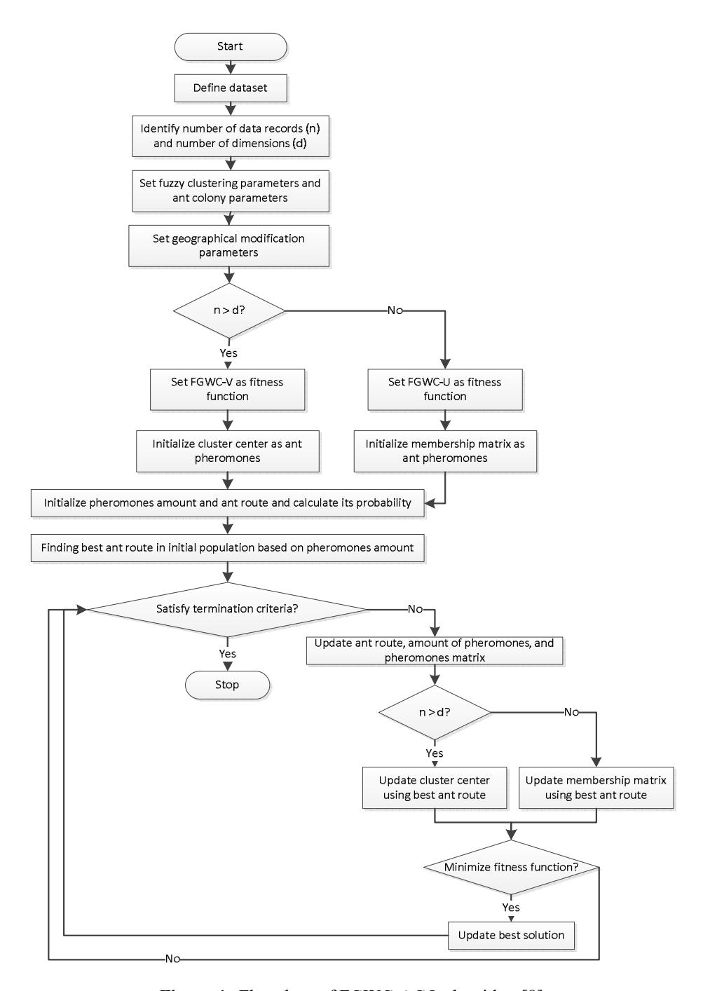
Figure 1 Flowchart of FGWC-ACO algorithm [8].

The membership matrix is modified by applying the population number, the geographical distance effect to calculate geo-demographic clusters, and the geographical weight in each clustering looping [5,8], as defined in Eq. (3) below:

\[u_i' = \alpha u_i + \beta \cdot \frac{1}{4} \sum_{j}^{n} w_{ij} u_j \tag{3}\] where \[\alpha + \beta = 1\] (4)

and \[w_{ij} = \frac{\left(m_i m_j\right)^b}{d_{ij}^a} \tag{5}\] where \(u_i\) is a new cluster membership degree in area i and \(u_i\) is the old cluster membership degree in area i. Variable \(w_{ij}\) is a weighting measure showing the effect of area i on j. \(\alpha\) and \(\beta\) are scale variables to affect the proportion between original membership and weighted membership, as expressed in Eq. (4). Parameter A is defined to ensure that the sum of the membership values of an area for all clusters is equal to 1. The weight is defined by the distance between the area center and the population of both areas, as shown in Eq. (5). Variable \(m_i m_j\) is the population number of area i and j, \(d_{ij}\) is the distance between i and j, and a and b are parameters defined by the user [5].

The minimized basic objective function of FGWC-ACO is expressed in the following equation (Eq. (6)) [8],

\[J_{FGWC-ACO}(U,V;X) = \sum_{i=1}^{c} \sum_{k=1}^{n} u_{ik}^{m} |v_{i} - x_{k}|^{2} \to min\] (6)

where m is a weighting exponent that determines the fuzziness of the cluster, \(u_{ik}\) is an element of the partition matrix, \(v_i\) is a cluster center, and \(x_k\) is a data point.

The FGWC-ACO algorithm uses modification of the basic objective function as shown in Eq. (6) to make it more optimal. The basic objective function is modified into two objective functions to handle the different datasets according to their size [16]. If for a dataset with n records and d dimensions n > d then the objective function calculation uses the cluster center \((J_{FGWC-ACO}(V;X))\), but if n < d, the calculation will be simpler by using the membership matrix for the objective function calculation \((J_{FGWC-ACO}(U;X))\) (See Eqs. (7) and (8)) [16].

\[J_{FGWC-ACO}(V;X) = \sum_{i=1}^{c} \sum_{k=1}^{n} \frac{|v_i - x_k|^2}{\left(\sum_{j=1}^{c} \left(\frac{|v_i - x_k|}{|v_j - x_k|}\right)^{\frac{2}{m-1}}\right)^m} \to min\] (7)

\[J_{FGWC-ACO}(U;X) = \sum_{i=1}^{c} \sum_{k=1}^{n} u_{ik}^{m} \left| \frac{\sum_{k=1}^{n} u_{ik}^{m} x_{k}}{\sum_{k=1}^{n} u_{ik}^{m}} - x_{k} \right|^{2} \to min\] (8)

To reach the global optimum solution in the initial phase, the FGWC algorithm is optimized using ACO. This metaheuristic method is inspired by ant colony behavior [17]. ACO uses the way ants find the shortest path to a food source and back to the nest. They find food by exploring the area around their nest randomly and then evaluate the quantity and quality of the food if they find it before bringing it to the nest. When they return to the nest, they will leave a pheromone on the ground based on the quantity and quality of the food they found. This pheromone will be used as a trail and will guide other ants to trace the food source [17].

2.2 Context-Based Clustering

Context-based clustering is a method that concentrates the original dataset by specific conditions from its dimensions, so only a subset of the original dataset with a suitable relation to the defined condition will be invoked [9,10,18].

For dataset N with attributes \(X = \{X_1, \dots, X_N\}\). The dataset is classified into C clusters in dimension space \((X \in R^r)\) with \(X_k\) is the k-th data point and \(V_i\) is the i-th cluster center. The context variable is defined with \(Y \in X\) (See Eq. (9)).

\[A: Y \rightarrow [0,1]\]

\[y_k \to f_k = A(y_k) \tag{9}\] where \(f_k\) represents the relation level between the k-th data point and the i-th cluster. To define the correlation between \(f_k\) and the membership of the k-th data point in the i-th cluster, the sum operator or the maximum operator can be used (See Eqs. (10) and (11)).

\[\sum_{i=1}^{c} u_{ki} = f_k; \ k = \overline{1,N} \tag{10}\]

\[\max_{j=1}^{C} u_{kj} = f_k; \ k = \overline{1,N}\] \[\tag{11}\]

For partition matrix U is defined in Eq. (12) as follows:

\[\text{[rumus tidak dapat ditampilkan dengan baik — lihat PDF asli]}\] \[\text{[rumus tidak dapat ditampilkan dengan baik — lihat PDF asli]}\] (12)

Steps to conduct the context-based clustering method [9,10,18]:

• 1. Initiate matrix U(t) at t = 0.
• 2. Recalculate center of each cluster according to Eq. (1).
• 3. Recalculate matrix U(t + 1) as provided in Eq. (13).

\[u_{ik} = \frac{f_k}{\sum_{j=1}^c \left(\left|\frac{v_i - x_k}{v_j - x_k}\right|\right)^{\frac{2}{m-1}}}; k = \overline{1, N}; i = \overline{1, C}\] \[(13)\]

4. Adjust partition matrix using geographical characteristics according to Eq. (3).

The method can make the algorithm's running time shorter because points with \(f_k\) equal to 0 will not be included in the calculation of the cluster centers and the membership degrees. Those points have no meaning within the defined context.

2.3 CUDA Parallel Programming

Compute Unified Device Architecture (CUDA) is a technology developed by NVIDIA to facilitate utilization of GPUs for general (non-graphic) purposes. CUDA is an architecture for parallel computing on a GPU, which makes it possible to develop and implement parallel programming algorithms on a GPU [19]. One can create programs that run on a GPU using a common programming language, such as C/C++ [20,21].

The CUDA program is divided into a host program, which consists of one or more consecutive threads that run on the host CPU, and one or more parallel kernels that are executed on a parallel processing tool like GPU [20,21]. Running CUDA starts with the execution program on the host CPU when kernel functions are called and then the execution moves to the GPU tool, where a large number of threads will be produced [20], as shown in Figure 2.

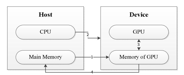
Figure 2 Basic architecture of CUDA [22].

Figure 2 illustrates the basic architecture of CUDA with the following process:

• 1. Copy input data from main memory to memory of GPU.
• 2. Program on host instructs program on GPU to run.
• 3. Execute parallel program in every core of GPU.
• 4. Copy result of parallel programming from memory of GPU to main memory.

2.4 Classification Entropy (CE) Validity Index

One clustering validity index that can be used to measure clustering quality is the classification entropy (CE) index. The CE index measures the fuzziness degree of a cluster partition, defined in Eq. (14) as follows [23,24].

\[CE = -\frac{1}{N} \sum_{i=1}^{c} \sum_{j=1}^{N} u_{ij} log_a(u_{ij})\] (14)

where \(u_{ij}\) is the membership of the j-th data point in the i-th cluster, N is the number of data points, and c is the number of clusters. The value range of the CE index is between \([0, \log_a c]\). The optimal number of clusters is in the minimum value of CE. The closer the CE index gets to 0, the better the clustering quality.

3 Proposed Method

In this research, the FGWC-ACO algorithm implemented in CUDA is denoted as FGWC-ACO-CUDA and CFGWC-ACO implemented in CUDA is denoted as CFGWC-ACO-CUDA. Two strategies are used. The first strategy is parallel computing implemented in the stage of solution evaluation, which is part of the clustering algorithm, FGWC. The second strategy is parallel computing implemented in the stage of both solution construction and solution evaluation. In the stage of solution construction, parallel computing is implemented in the pheromone updating when constructing the solution in the form of a cluster center or a membership matrix. In implementation, the first strategy is denoted as CUDA-1 and the second one is denoted as CUDA-2. In this research, the results of implementing CUDA using these two strategies were compared.

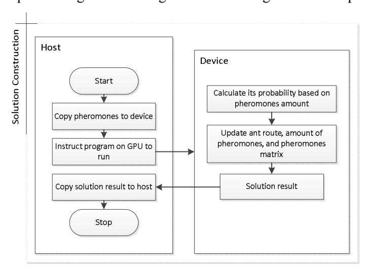
Figure 3 CUDA implementation in solution construction.

Implementation of CUDA parallel programming is done in the stage of solution construction and solution evaluation. The steps of implementing CUDA in the stage of solution construction and solution evaluation are illustrated in Figures 3 and 4 using flowcharts.

The first step in the solution construction stage is to copy the pheromones initialized in the host to the device. Then for every thread, solution construction is conducted based on the amount of pheromones and its probability is calculated. Then the ant route, the amount of pheromones and the pheromone matrix are updated. The pheromone matrix is a solution that has a size based on the population size and the problem dimension. After all threads have finished their task, the solution result is copied to the host.

Solution evaluation is divided into two, as follows. If n < d then the FGWC-U function is used with the membership matrix as input. If n > d then the FGWC-V function is used with the cluster center as input.

Steps of CUDA implementation in FGWC-U:

• 1. Copy clustering parameter and geographical parameter from host to device.
• 2. Copy membership matrix as input data to device; this is the solution that is produced from the stage of solution construction.
• 3. For every thread, calculate every element of weight for geographical modification.
• 4. For every thread, calculate every element of the cluster center.
• 5. For every thread, calculate membership matrix and membership matrix with geographical modification.
• 6. Check whether it reaches the termination criteria. If yes, copy cluster center and membership matrix to host. If not, back to step 4.

Steps of CUDA implementation in FGWC-V:

• 1. Copy clustering parameter and geographical parameter from host to device.
• 2. Copy cluster center as input data to device; this is the solution that is produced from the stage of solution construction.
• 3. For every thread, calculate every element of weight for geographical modification.
• 4. For every thread, calculate membership matrix and membership matrix with geographical modification.
• 5. For every thread, calculate every element of the cluster center.
• 6. Check whether it reaches the termination criteria. If yes, copy cluster center and membership matrix to host. If not, back to step 4.

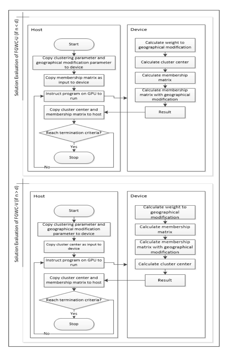
Figure 4 CUDA implementation in solution evaluation.

Using CUDA parallel programming for the FGWC-ACO algorithm has the same procedure as using CUDA for the CFGWC-ACO algorithm. The only difference is in the step of calculating the membership matrix. When calculating the membership matrix in the CFGWC-ACO algorithm, it has a modified formula using a defined context variable.

4 Experimental Result

An experiment was done to compare the running time of the original algorithm and that of the proposed algorithm by calculating the average of 50 running times of each algorithm. The algorithms were run on Windows 8 64 bit with Intel® Core™ i5-4200U CPU @ 1.6GHz 2.3GHz, 4GB RAM.

This experiment was done using three datasets taken from the Indonesia Population Census 2010 with different sizes. The first dataset contained regency-level data from one province, consisting of 14 data points; the second contained provincial-level data, consisting of 33 data points; and the third one contained regency-level data from one island, consisting of 118 data points. This dataset contains 110 social-demographic variables [25]. The clustering parameters were defined as fuzziness exponent m = 2, δ = 0.001, and geographic parameters were defined as α = 0.5, β = 0.5, a = 1, and b = 1.

Figure 5 shows the experimental result of using CUDA parallel programming for the FGWC-ACO algorithm. Implementation of CUDA in the stage of solution evaluation shows that the running time was shorter than that of the FGWC-ACO algorithm. In FGWC-ACO-CUDA-1, implementation of CUDA was done in the stage of solution evaluation, which is a process from the FGWC algorithm, so the process of sending data from the host to the device and vice versa only happens in the clustering process. This clustering process happens in each ACO iteration, so the running time of FGWC-ACO-CUDA-1 was shorter than that of FGWC-ACO, but it still increased because of the number of clusters defined. So, the acceleration result of FGWC-ACO-CUDA-1 was not maximal.

The acceleration produced by comparing the running time of FGWC-ACO with that of FGWC-ACO-CUDA-1 is shown in Figure 6. Based on the experimental result, the acceleration produced by the dataset with size 14 was up to 2.4 times, the dataset with size 33 produced an acceleration of up to 3 times, and the dataset with size 118 produced an acceleration of up to 3.5 times.

In FGWC-ACO-CUDA-2, implementation of CUDA is not only done in the stage of solution evaluation, but also in the stage of solution construction. The solution construction process happens in each ACO iteration, and so does the

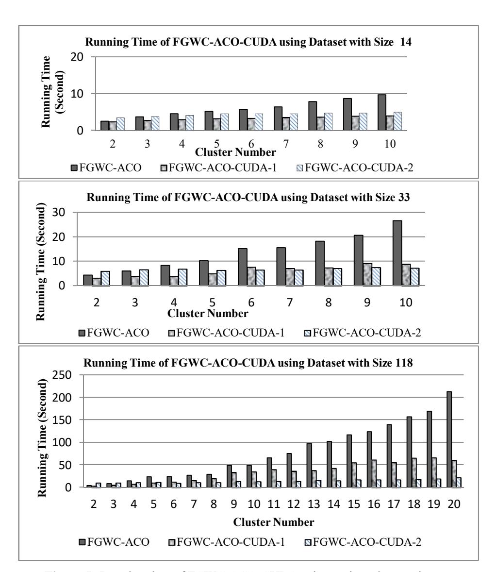
Figure 5 Running time of FGWC-ACO-CUDA using various dataset sizes.

evaluation process. More processes running in parallel means that the running time produced will be shorter. On the other hand, more parallel processes run by CUDA kernels means that more time is needed to send data from the host to the device. This causes a speed reduction in processes with a small number of clusters. If the number of clusters is large, it is not too influential because sequential processing on large numbers of clusters needs more time. Based on the experimental result, the acceleration produced by the dataset with size 14 was up to 1.9 times, the dataset with size 33 produced an acceleration of up to 3.6 times, and the dataset with size 118 produced an acceleration of up to 9.8 times.

Figure 7 shows that FGWC-ACO-CUDA-2 decreases the amount of running time on cluster numbers 1 and 2, and the speed increased along with the increase in number of clusters. From the acceleration produced by FGWC-ACO-CUDA-1 and FGWC-ACO-CUDA-2 it can be concluded that for small datasets or small cluster numbers, the running time is shorter when using the FGWC-ACO-CUDA-1 algorithm. Otherwise, for large datasets or large cluster numbers, using the FGWC-ACO-CUDA-2 algorithm further increases the algorithm's performance. Figure 8 illustrates that an increase in performance using CUDA parallel programming does not change the clustering result. The CE index value for the FGWC-ACO algorithm is the same as the CE index value for the FGWC-ACO-CUDA algorithm. Implementation of CUDA in the CFGWC-ACO algorithm shows a result with the same characteristics as the result of the implementation of CUDA in the FGWC-ACO algorithm.

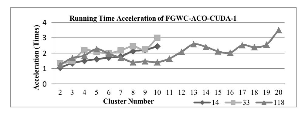
Figure 6 Acceleration time of FGWC-ACO-CUDA-1 based on dataset sizes.

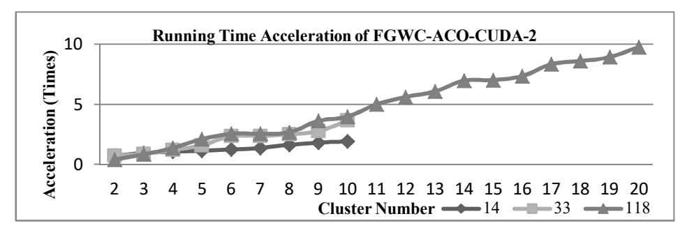
Figure 7 Acceleration time of FGWC-ACO-CUDA-2 based on dataset sizes.

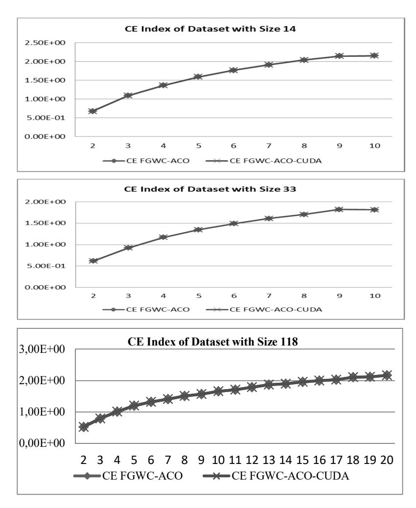
Figure 8 CE validity index of FGWC-ACO-CUDA algorithm.

5 Conclusion

In this paper, implementation of CUDA parallel programming for the FGWC-ACO and CFGWC-ACO algorithms was proposed in order to optimize the running time of the FGWC-ACO algorithm. In the implementation of CUDA parallel programming, the experimental result proved that it is able to increase the running time speed. In the experiment, the maximum acceleration that was reached was up to 9.8 times. Evaluation of clustering quality after implementing CUDA parallel programming had the same result as with the original algorithm because both algorithms produce the same membership matrix and cluster centers. Future research that can be done is to investigate how to implement

CUDA parallel programming by applying a multi-GPU device, so a higher increase of computation speed can be reached. As in our previous paper [12], one context variable was used in this research. It is an interesting challenge to implement two or more context variables when conducting context-based clustering so the result can focus on the correlation between two or more context variables. Beside that, in the clustering process, it will be useful to build a tool to interpret and visualize new information from the clustering data, especially when applying clustering to large datasets.