
1 Introduction
Available bandwidth estimation schemes or tools have been developed recently as support mechanisms in various fields, for example to maintain compliance of service level agreements, network management, data traffic engineering, providing resource for real-time application, congestion control, to detect failures and attacks on networks, and admission control [1]. Available bandwidth estimation is an important component of the mechanism of admission control for providing quality of service (QoS) on wireless and wired networks. Furthermore, available bandwidth estimation in wireless local area network (WLAN) environments is one of the important and effective functions for network resources management and service provisioning that can guarantee QoS of multimedia real-time applications [2]. It can be used as one of the parameters to adjust video or audio quality while they are being transmitted. For example, when the available bandwidth is sufficient, both audio and video quality can be enhanched. On the other hand, when the available bandwidth is not sufficient, the quality of one of some multimedia components can be enhanched while the quality of others is lowered.
This paper presents our work on the development of an available bandwidth estimation technique based on existing techniques, i.e. Distributed Lagrange Interpolation Based Available Bandwidth Estimation (DLI-ABE) [3] and Accurate Passive Bandwidth Estimation (APBE) [4]. The idle-period synchronization model in APBE uses parameters of various node conditions at optimal workload instead of node state synchronization between the sender and receiver nodes, which can be affected by other nodes. Optimal workload is the point where the network achieves the best performance without interference from other nodes [5]. Therefore, the proposed passive measurement scheme was developed with the involvement of the relevant calculation of actual channel utilization and collision probability caused by data flow from hidden nodes. In addition, actual channel utilization can be influenced by several other factors, for example, proportion of distributed coordination function interframe space (DIFS) duration, backoff delay, acknowledgment delay, synchronization of various conditions of sender and receiver nodes, as well as traffic from hidden nodes. DIFS is the waiting time before the sender starts transmitting data frames after completing backoff [6].
Furthermore, the proposed scheme in this research was validated by comparing it with the existing DLI-ABE and APBE schemes. Estimations of these three schemes were compared with actual available bandwidth. Their performance was analyzed based on two metrics, i.e. level of accuracy and error estimation. Validation of the proposed scheme was conducted based on a simulation using the OMNet++ network simulator.
The rest of this paper is organized as follows. Section 2 explains related work on approaches or schemes to estimate available bandwidth in a network. Section 3 explains our proposed scheme to estimate available bandwidth based on calculation of idle-period synchronization between sender and receiver nodes and packet collision probability caused by data flow from hidden nodes. Section 4 explains the experimental scenario used to analyze the performance of the proposed available bandwidth scheme. Section 5 explains the performance comparison of the proposed scheme with other schemes. Section 6 discusses available bandwidth estimation in wireless networks and our proposed scheme. Finally, we conclude this paper in Section 7.
2 Related Works
Many research works focus on the development of available bandwidth estimation because this is one of the crucial functions for the effective management of network resources and services provision that can guarantee QoS of real-time multimedia applications, especially in 802.12 wireless networks with limited bandwidth [7]. Research works on available bandwidth estimation techniques can be broadly classified into two main categories, i.e. active probing and passive measurement [7,8]. Tools that have been developed based on active probing approaches are for example, Spruce [9], Initial Gap Increasing (IGI) [10], Pathload (Jain and Dovrolis [11], and Pathchirp [12]. Schemes that were developed based on passive measurement approaches are for example, Adaptive Admission Control (AAC) [13], Cognitive Passive Estimation of Available Bandwidth (cPEAB) [14], Accurate Passive Bandwidth Estimation (APBE) [4], and Distributed Lagrange Interpolation Based ABW Estimation (DLI-ABE) [3].
2.1 Active Probing Approaches
Generally, bandwidth estimation approaches that depend on active probing mechanisms send probe packets over the network using various traffic rates. The available bandwidth can be calculated from the probing rate that can be managed in different ways by analyzing the packet inter-arrival delay [17]. By determining the delay experienced by probing packets transmitted through tight links, the available bandwidth can be determined.
In their study, Hu, et al. [10] have proposed IGI. Research by Santander [15] showed that the IGI algorithm transmits a packet sequence train to the destination node by increasing the initial gap. This gap is used to estimate the level of cross traffic in the link. Cross traffic is the existing transmission of data packets [16]. Then, IGI provides an estimation of the available bandwidth after a certain amount of cross traffic has been subtracted from the known bottleneck link capacity [10]. In another study, Strauss, et al. [9] proposed an available bandwidth estimation technique called Spruce. The authors concluded that Spruce is more accurate than Pathload and IGI. Ribeiro [12] has proposed Pathchirp. Pathchirp uses the same principle of self-induced congestion as used in Pathload. However, Pathchirp does not transmit packet trains (or streams) at a certain rate as Pathload does but increases the rate at every train probing exponentially.
Active probing approaches has disadvantages because they can generate additional traffic information such as packet loss, jitter, and delay [17]. However, such schemes generate additional traffic load to the network, which may cause performance degradation of existing flows [17]. Moreover, they take
long time for the measurements and produce lower accuracy compared to other bandwidth estimation techniques [14,17].
2.2 Passive Measurement Approaches
The main concept of passive measurement approaches is to monitor the traffic that already exists in a network and estimate available bandwidth. This type of approach is also known as calculation-based techniques [7] because they do not insert a probe packet to calculate the available bandwidth. In contrast to active probing techniques, passive measurement techniques estimate the available bandwidth by monitoring traffic conditions based on the ratio of the use of the channel and provide an alternative way to evaluate the available bandwidth without affecting the traffic flow in the existing network [17].
Sarr, et al. [18] proposed an enhancement of Available Bandwidth Estimation (ABE). ABE is a technique to calculate the available bandwidth between two neighbor nodes along a path. This technique involves transmission radius, medium monitoring to estimate medium occupancy of each node, combination of these values to calculate state synchronization between nodes, overhead impact estimation, and estimation of collision probability between each pair of nodes. [18].
In a recent work on a passive measurement based approach, the Accurate Passive Bandwidth Estimation (APBE) scheme [4] is proposed. APBE considers a factor that is ignored in cPEAB, the RTS (request to send) and CTS (clear to send) overhead in estimating available bandwidth. Eq. (1) represents the available bandwidth estimation of APBE:
\[AB_{APBE} \approx (1 - K)(1 - R/C)(1 - ACK)(1 - P_c)\frac{T_i}{T}C\] (1)
where K is the proportion of bandwidth consumed by waiting time and the backoff mechanism, R/C is the overhead caused by the RTS and CTS procedure, ACK is the proportion of the bandwidth consumed by the acknowledgement mechanism (acknowledge frame transmission), Pc is the collision probability as the impact of flows by hidden nodes, Ti is the channel idle time, and C is the maximum capacity of the channel. Channel idle time as used in APBE only considers the channel idle time on the sender and receiver nodes but does not take into account the transmission of data packets from other nodes that can affect the states of both the sender and receiver nodes.
Another passive available bandwidth estimation method is Distributed Lagrange Interpolation Based ABW Estimation (DLI-ABE), as proposed in Chaudhari, et al. [3]. DLI-ABE is a scheme that estimates available bandwidth in a network by using passive measurement based on idle-period synchronization, collision
probability based on packet length and random waiting time. DLI-ABE uses a random waiting time (K) coefficient that is calculated based on the backoff time, the short inter-frame space (SIFS) and DIFS duration, the delay required for the RTS/CTS mechanism and the acknowledgment delay that use the channel.
Furthermore, DLI-ABE calculates collision probability (Pm) as an impact from packet length. It can be obtained by Eq. (2).
\[P(m) = (f(m) \times p_{Hello}) \tag{2}\] where f(m) is a Lagrange Interpolation polynomial and phello is the hello packet collision probability of any packet of size (m), the same as used in ABE.
DLI-ABE estimates the available bandwidth on the link between the sender and receiver nodes using idle-period synchronization, probability of collision, and random waiting time based on Eq. (3).
\[AB_{DLI-ABE} \approx (1 - K)(1 - P_m) \left( \min \left( \left[ \frac{T_i^{S}(1 - p(T_s^{T}/T))}{T} \right] C, \left[ \frac{T_i^{T}(1 - p(T_s^{S}/T))}{T} \right] C \right) \right)\](3)
3 Proposed Available Bandwidth Estimation Scheme
In our proposed scheme, we focus on passive measurement technique. However, as in [17] in addition to the medium occupancy ratio, the following issues are also involved:
- 1. Node state synchronization between the sender and receiver nodes.
- 2. Overhead probability by control message mechanisms in the MAC layer.
- 3. Packet collision probability, which consists of the following lists: a. packet collision probability caused by neighbor nodes; b. packet collision probability caused by hidden nodes.
3.1 Hidden Nodes
The hidden-node problem is illustrated in Figure 1, which shows three nodes (node A, B, and C). Node B is within the transmission range of nodes A and C, whereas node C is located outside the transmission range of node A. In a situation like this, node C cannot detect transmission from node A and consequently it can indirectly interfere with node B's reception of A's transmission [19].
The transmission range of a node A is defined as the area in which the surrounding nodes can receive packets from node A. Whereas the carrier sense of node A can be perceived, it cannot be used to receive transmitted packets [19].
Figure 1 Hidden node.
To solve the hidden-node problem, several methods or techniques can be implemented. Each solution is suitable for a particular scenario, i.e. increasing transmitting power from the nodes, using omni-directional antennas, removing obstacles, moving the nodes, using protocol enhancement software, using antenna diversity, and using a wireless central coordinated protocol [20].
3.2 Calculation of Idle-period Synchronization
As described in Section 2, APBE considers channel idle time on the sender and receiver nodes, but it does not take into account the transmission of data packets from other nodes that can affect the state or condition of both the sender and the receiver node. However, Chaudhari, et al. [3] state that the medium on the sender node must be in free condition, so that the medium can be accessed to transmit data packets. In addition, at the same time the receiver node must also be in free condition during the time required to transmit whole data packets, in order to avoid collisions. Both conditions are provisions to estimate the available bandwidth accurately. Furthermore, the medium condition of a node can be influenced by the flow of data packets originating from other nodes. Based on these assumptions, the idle condition of the sender and receiver nodes should be synchronized so that communication can be established. Therefore, in this research we adopted idle-period synchronization between the sender and receiver nodes as used in DLI-ABE.
The channel state perceived by the sender and receiver nodes helps to find idleperiod overlap between the sender and receiver nodes. In practice, a node has three channel conditions, i.e. BUSY, SENSE BUSY, and IDLE [3]. The author of APBE only considered the channel IDLE time used in the calculation to estimate available bandwidth and did not involve the BUSY and SENSE BUSY states. However, by distinguishing these two time periods, we can obtain information ahout how they can affect the synchronization state of the sender and receiver nodes, and consequently on the estimation of idle-time overlap and available bandwidth [5].
A node is in BUSY state when the channel is transmitting or receiving data packets. It is in SENSE BUSY state when the node senses that the channel is busy, but no frames are being received. A node enters the state of sensing when the medium is sensed as busy but no frames are being received because the energy level is below that of receiving [5]. In other words, the channel is in SENSE BUSY condition when a node is not transmitting or receiving any frames of data packets, but there is another node that is sending or receiving frames of data packets and is located within the first node's carrier sense range. In addition, any other state not included in both conditions is defined as IDLE state.
Before further discussion of idle-period synchronization, we will first explain the concept of probability of idle-time overlap between the sender and receiver nodes. Overlap is a condition in which the channels on the sender and receiver nodes are in the same condition (busy or idle). For example, Figure 2 represents a possible idle-period overlap between the sender and receiver nodes [3,5].
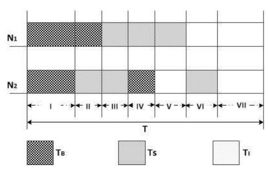
Figure 2 Channel occupation phase.
In Figure 2, N is node, TB is time duration of BUSY state, TS is time duration of SENSE BUSY state, and TI is time duration of IDLE state. Furthermore, all periods in Figure 2 encounter overlap, except at periods V and VI. At periods V and VI, the available bandwidth will decrease because of the non-overlap of the idle times between the sender (s) and receiver (r) nodes [3]. During this period, one of the nodes is in SENSE BUSY state while the other node is in IDLE state [3]. DLI-ABE uses these two periods to find the idle-period synchronization at the sender and receiver nodes. As in [5], the duration of the IDLE state in a node can be obtained by Eq. (4):
\[T_i = T - T_B - T_S \tag{4}\] where T is measurement period.
Like DLI-ABE, our proposed scheme uses the p coefficient to represent the probability that s is in SENSE BUSY state and r is in IDLE state or, conversely, the probability that r is in SENSE BUSY state and s is in IDLE state. Furthermore, the proposed scheme uses the actual channel utilization and the collision rate. Eqs. (5) and (6) are used to calculate idle-period synchronization at the sender node (\(T_s\)) and the receiver node (\(T_r\)) using their various states [3,7].
\[T_{s} = \left\lceil \frac{T_{i}^{s}(1 - p(T_{s}^{r}/T))}{T} \right\rceil \tag{5}\]
\[T_r = \left\lceil \frac{T_i^T (1 - p(T_s^S/T))}{T} \right\rceil \tag{6}\]
In Eqs. (5) and (6), \(T_i^s\) is the IDLE duration of the sender node, \(T_i^r\) is the IDLE duration of the receiver node, \(T_s^s\) is the SENSE BUSY duration of the sender node, \(T_s^r\) is the SENSE BUSY duration of the receiver node, and p is the collision rate experienced by a node. As in Zhao et al. [5], assuming that the nodes are distributed uniformly in a dense network, we used the p coefficient value equal to 0.66.
3.3 Possible Overhead on MAC Layer
The general IEEE 802.12 basic frame exchange sequence is depicted in Figure 3 [14]. At Interval I, the medium is sensed as being in busy condition. If in this interval there is interference (interruption) during DIFS, the transmission process is returned and restarted completely when the medium is back to idle condition. In other words, when the sender node wants to transmit new packets, it needs to monitor the channel first. If the channel is sensed to be idle for a period of time equal to DIFS, it begins the transmission. Otherwise, if the channel is busy (either immediately or during DIFS), the station persists to monitor the channel until it is measured idle for a period of time equal to DIFS. At this point, the station will generate a random number of backoff slot time based on the contention window (CW) size before transmitting, in order to minimize the probability of collision with packets being transmitted by other stations. During the backoff procedure, if the channel is idle for a period of time equal to DIFS, the backoff timer is decremented as long as the channel is sensed idle. The backoff timer will be stopped or paused when a transmission is detected on the channel and will be resumed when the channel is sensed idle again for more than a period of time equal to DIFS [21]. Backoff is calculated in the sender node.
Interval I is a kind of throughput overhead to reduce inaccuracies in estimating available bandwidth. Therefore, we adopted the K coefficient as used in Park, et al. [4] and Tursunova, et al. [17], which represents the proportion of bandwidth consumed by DIFS time and the backoff mechanism.
The backoff time is a changing variable, therefore we use its average value \((\overline{backoff})\) as in Tursunova et al. [17] when calculating the K coefficient. K is obtained by Eq. (7):
\[K = \frac{DIFS + \overline{backoff}}{T} \tag{7}\]
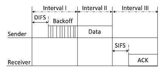
Figure 3 IEEE 802.11 frame exchange sequence (Tursunova, et al. [17]).
In Eq. (7), backoff is the waiting time of medium access control at a node in the network before transmitting data packets or retransmitting a frame after a collision occurred, while T is the measurement period.
In addition, receiver node waits for a short inter-fame space (SIFS) interval when it receives the data packet correctly and then transmits an acknowledgement (ACK) message to the sender node [21]. The sender node is considered to have failed on the previous transmission if it does not receive the ACK and then schedules to retransmit the data packet [21]. Average backoff is calculated from the sender's IEEE 802.11 radio that is going to transmit the data packets. The radio can the sense interference signals from other nodes, so that data packets will be delayed (backoff) until the medium is in idle condition (no interference). The backoff method requires each node to choose a random number (n) between 0 contention window (CWmin) and will wait for this number of slots to decrease before accessing the medium. The backoff method also requires each node to check whether other nodes have accessed the medium before. Slot time is set so that a node will always be able to determine if another node has accessed the medium at the beginning of the previous slot. This can reduce the probability of collision between packets by half. Exponential backoff is triggered each time a node chooses a slot and collision occurred. This condition increases the maximum number for random selection exponentially [22]. If the data packet is not transmitted successfully, CWmin will be doubled until it reaches the maximum value (CWmax) [21].
The proposed scheme also assumes that the delay acknowledgment (ACK) acts as control message overhead as in Park, et al. [4] and Tursunova, et al. [17]. Although the proportion of bandwidth used by the acknowledgment procedure is not large, it still has an impact on the estimated available bandwidth. Furthermore, by eliminating overhead, estimation of the available bandwidth
becomes more accurate. ACK is the proportion of MAC delay that can be obtained by Eq. (8) [17]:
\[ACK = \frac{ACKTimeout + SIFS}{T} \tag{8}\]
3.4 Packet Collision Probability
In wireless networks, interference of data packet transmission can occur, particularly if there are multiple nodes that are adjacent to each other. This is because the transmission channel or medium is shared by a number of nodes. This can cause QoS degradation, which has an impact on the performance of the link, for example, a higher error ratio while transmitting or receiving data packets, higher packet collision, more delay, and so on. In a wireless network, adjacent nodes that are close to each other can be categorized into two types, i.e. exposed nodes and hidden nodes. These two types of nodes have different effects on data transmission in wireless links [23]. Furthermore, based on Tay [24] and Tursunova, et al. [17], packet collision probability can be affected by neighbor nodes, which is based on the number and position of these nodes.
3.4.1 Packet Collision Probability Caused by Number of Neighbor Nodes
Wireless networks are highly vulnerable to collision problems. The possibility of collision occurs when a node (e.g. node A) starts transmitting data packets and these data packets collide with data packets transmitted by another node (e.g. node B). As described in Section 2, DLI-ABE states that packet collision probability depends on packet length. However, according to research conducted by Tay [24], the probability of packet collision does not depend on packet length but only on number of neighbor nodes (number of neighbor nodes that are trying to access the same medium) and average backoff window size (control access to the medium).
Tursunova, et al. [17] assumed that when there are enough other stations or nodes so that the transmission from node A and node B cannot be synchronized (for example, on an EDCA network), then node A can start transmission anytime. Based on these assumptions, the transmission of data packets from node A has the possibility to collide with data packets transmitted by node B, where the possibility of collision can be obtained by 1/backoff.
In addition, if there is a network system that consists of n nodes that are adjacent or neighboring to node A or if they are connected to the same AP (access point), then the probability of node A colliding with another node can be obtained by Eq. (9) [17, 24]:
\[P_{coll} = 1 - \left(1 - \frac{1}{\overline{W_{backoff}}}\right)^{n-1} \tag{9}\]
In Eq. (9), \(\overline{W_{backoff}}\) is average backoff window size. Moreover, similar to the calculation of the K coefficient, the calculation of \(\overline{W_{backoff}}\) used in Eq. (9) above is a variable that is changing as well, therefore we use its average value to calculate \(P_{coll}\).
3.4.2 Packet Collision Probability Caused by Hidden Nodes
The probability of packet collision can be caused by data flow from multiple nodes. For instance, data packets are being transmitted from node A to node B, but there is a hidden node that currently transmits data packets as well. Then node A has the possibility of having a collision, which leads to loss of data packets transmitted.
DLI-ABE does not consider the impact of data packets transmitted from hidden nodes. This causes the estimated available bandwidth result by DLI-ABE to be inaccurate. Moreover, according to the research conducted by Wei [23] and Tursunova, et al. [14], the probability of collision between packets is closely related to the data flow from hidden nodes. In other words, the probability of collisions will also increase when the data flow is greater. Based on this, the probability of collision caused by data flow from hidden nodes can be calculated by Eq. (10) [17]:
\[P_c = \begin{cases} \frac{f_-h}{c}, & if \left(0 \le \frac{f_-h}{c} \le 1\right) \\ 1, & otherwise \end{cases}\] (10)
Based on Eq. (10), f h is the total throughput of hidden nodes.
Then, based on Eqs. (9) and (10), the collision probability can be calculated by using Eq. (11) [17]:
\[P_c = (1 - P_{coll}) \times (1 - P_h)\] (11)
3.5 Available Bandwidth Estimation Using Proposed Scheme
The proposed scheme estimates the available bandwidth at the link between the sender and receiver nodes using idle-period synchronization, collision probability, and possible overhead by control messaging that may occur. Based on Eqs. (5) to (8), and (11), we propose that the available bandwidth (AB) estimation scheme can be estimated using Eq. (12):
\[AB \approx (1 - K) \times (1 - ACK) \times P_c \times (min([T_s \times C], [T_r \times C]))\] (12)
where C is maximum channel capacity.
Based on Eq. (12), we propose a scheme to estimate the available bandwidth on wireless networks. The scheme involves four parts: the random waiting time before the data packet is transmitted; the delay or transmission time for the acknowledgment frame; the probability of collision between data packets transmitted from various nodes; and node state synchronization between the sender and receiver nodes.
The random waiting time (K) is calculated based on DIFS and average backoff time. Delay acknowledgment (ACK) acting as a control message is calculated based on acknowledge frame transmission timeout and SIFS overhead. The packet collision probability (Pc) is calculated based on two factors, i.e. the number of nodes and the position of these nodes. Node state synchronization is calculated based on the model for idle-period synchronization at the sender and receiver nodes. Moreover, the available bandwidth for the end-to-end network path that consists of multiple links is estimated as the minimum available bandwidth among these multiple links.
4 Experimental Setup
In this section, we describe the experimental setup to analyze the performance of the proposed available bandwidth estimation scheme. This includes choosing the measurement period, developing a network simulation model, and proposing the validation method.
4.1 Choosing Measurement Period
The available bandwidth is estimated every T seconds. The studies conducted by Chaudhari, et al. [3], Park, et al. [4], and Tursunova, et al. [17] indicate that the sample period or the time required for estimating the available bandwidth must be small enough so that the available bandwidth scheme can react or respond quickly to changes in the wireless network. Therefore, for making a fair comparison with APBE and DLI-ABE, in this study we have chosen the same measurement period, which is T = 1 s. This scenario was also used by Tursunova, et al. [17] and Zhao, et al. [7].
4.2 Developing Simulation Model
As depicted in Figure 4, our network simulation model consists of four mobile nodes (MNs) and two access points (APs). The type of medium used in this research was IEEE 802.11g with 54 Mbps physical link capacity. The transmission power of the radio used was 0.009 mW. In addition, we set the signal attenuation threshold parameter at -57.5 dBm to represent the carrier sense range on each AP and MN. Based on this configuration, we obtained that MN 1 and AP 1, MN 2 and AP 1, MN 3 and AP 2, as well as MN 4 and AP 2 had the same distance, i.e. 11 m, while MN 2 and MN 3 had a 30-m range. In addition, each node had a carrier sense range of approximately 35 m.
Figure 4 Network model with hidden node.
This study developed a scenario where the available bandwidth was measured as throughput that still can be transmitted by AP 1 to the receiver node within its transmission range and had carrier sensing that could reach MN 3, but this node was located outside of MN 3's transmission range, so that the receiver node was affected by MN 3's data packet transmission. In this study, MN 1, AP 1, and MN 2 were connected to each other, as in Park, et al. [4], and MN 1 transmitted UDP data packets at 500 Kbps bitrate. Meanwhile, the traffic load sent by MN 3 increased from 1 Mbps to 7 Mbps at a 1 Mbps bitrate interval to MN 4 through AP 2. Both MN 1 and MN 3 were sending UDP data traffic with a packet size of 1024 bytes.
Based on Figure 4, when MN 3 is a node hidden to AP 1 and there is a flow of data from MN 3 to MN 4 through AP 2, then collisions between data packets may occur in MN 2. In other words, MN 2 can feel (sense) the data transmission from MN 3 but AP 1 cannot feel the transmission performed by MN 3. This yields a reduced amount of available bandwidth on the connected link between AP 1 and the receiver node, which can sense MN 3's transmission but is located outside of MN 3's transmission range.
AP1 and MN3 are 1-hop neighbor nodes of MN2. According to Wei [23], AP1 can be set to monitor data flow, record and update the flow information of 1 hop neighbor nodes periodically. For each node, it can receive data flow information from all of its 1-hop neighbor nodes, which means that it can obtain the flow information of all 2-hop neighbor nodes [23]. Based on Figure 4, AP 1 receives the data flow information from MN 2, broadcast by MN 2. As MN 3 is a 1-hop neighbor of MN 2, AP 1 can get the flow information of MN 3, and MN 3 is AP 1's 2-hop neighbor. Similarly, AP1 can get the data flow information from MN 1. So, AP 1 will be able to obtain the flow information of all of its 2 hop neighbors. Therefore, f_h can be calculated by subtracting MN 3 to AP 2 throughput from AP 1 to MN 2 throughput and MN 3 to AP 2 throughput.
4.3 Validation Method
The performance of the three schemes was measured based on two metrics, i.e. level of accuracy and error estimation. The accuracy metric is a quantitative measurement result that is obtained by comparing the estimated available bandwidth value by each of the available bandwidth estimation schemes with the expected (actual) value of available bandwidth in each test case. To measure the actual available bandwidth, we added two nodes that were used to transmit and receive data packets. We configured these additional nodes to transmit and receive data packet traffic that could saturate the wireless channel. In this study, we developed a scenario in which this traffic consisted of data packets that used the UDP protocol with a packet length of 1024 bytes. The data packet transmission rate from additional sender node to additional receiver node was adjusted to the data packet transmission rate from MN 1 to the MN 2. In our study, the maximum throughput of the data packet flow that could saturate the transmission medium obtained from the additional sender node's data flow to the additional receiver node without affecting (reducing throughput) the cross traffic (data flow from MN 1 to the MN 2), was the actual available bandwidth.
Then, the next metric to be compared was the measurement of the ratio of the estimated error level. The estimation error ratio indicates the error level of each technique tested against the actual or real available bandwidth. The estimation error ratio is closely related to accuracy. As in the research conducted by Chaudhari, et al. [3], Park, et al. [4], and Tursunova, et al. [17], the estimation error ratio can be obtained using Eq. (13):
\[Error Ratio = \frac{|RealAB - EstimatedAB|}{RealAB} \times 100\%\] (13)
where RealAB is the actual available bandwidth, whereas EstimatedAB is the estimated available bandwidth based on a certain available bandwidth estimation technique. To avoid mistakes and make it easier to interpret the error ratio, we used the absolute value. With the usage of this absolute value, any available bandwidth estimation error obtained based on each technique is a positive value.
5 Experimental Result Analysis
In this section, we describe a comparative analysis of each scheme's performance in estimating available bandwidth in a wireless network. The estimated available bandwidth results were obtained by an experiment conducted using the OMNet++ network simulator tool. The calculation results are depicted in Figures 5, 6 and 7.
From Figure 6 we found that when there were hidden nodes that generated traffic load from 1 Mbps to 4 Mbps or traffic load that consumed 52% of the maximum bandwidth capacity, the available bandwidth on the measured link would decrease significantly. However, when there was traffic load more than 4 Mbps from a hidden node or if it consumed more than 52% of the maximum bandwidth capacity, the maximum available bandwidth on the target link did not decrease significantly. Traffic load generated by hidden nodes ranging from 1 Mbps to 4 Mbps reduced the available bandwidth. Gradually decreasing from 5,754 Mbps, 5,007 Mbps, 4,172 Mbps to 3,775 Mbps on each traffic load, it was increased with average bandwidth consumption at approximately 0,65 Mbps. However, when the traffic load generated by hidden nodes was more than 4 Mbps, the available bandwidth did not significantly decrease. The availability of bandwidth, gradually decreasing from 3,775 Mbps, 3,576 Mbps to 3,431 Mbps on each traffic load, was increased with average bandwidth consumption approximately 0,18 Mbps.
Based on the estimated available bandwidth result obtained from the comparison of the three schemes in Figure 5, the estimation error rate of each scheme can be seen in Figures 6 and 7. The proposed scheme had an error rate that tended to decrease (is more accurate) when there was traffic load generated by hidden nodes ranging from 1 Mbps to 4 Mbps. This is similar to APBE's error rate. However, the proposed scheme had a lower estimation error rate when compared to APBE and DLI-ABE.
Based on Figure 7, we can see that our proposed scheme had the lowest estimation error rate compared with APBE and DLI-ABE. This shows that the proposed scheme has better accuracy to estimate the available bandwidth on a wireless network. This is because the APBE scheme does not involve synchronization of channel idle time on the sender and receiver nodes that can be affected by the busy condition from hidden nodes, called sense busy condition. Meanwhile, the DLI-ABE scheme considers packet size and packet loss to estimate available bandwidth. However, based on the experiment, the packet size does not affect the availability of bandwidth on the wireless network directly, while the collision can cause fluctuating packet loss changes, although traffic load generated by hidden nodes increases. These reasons cause the lack of accuracy of the two schemes that have been proposed previously.
In contrast to the two previous schemes, the proposed scheme estimates the available bandwidth by taking into account the traffic load generated by hidden
nodes as well as sense busy state at the receiver node that is affected by the hidden nodes. Therefore, based on the result of the estimated error rate statistics calculation, our proposed scheme can estimate available bandwidth on a wireless network approximately 0.9% more accurately when compared to APBE and 21.8% more accurately when compared to DLI-ABE. In other words, the proposed scheme can estimate the available bandwidth more accurately than both other existing schemes.
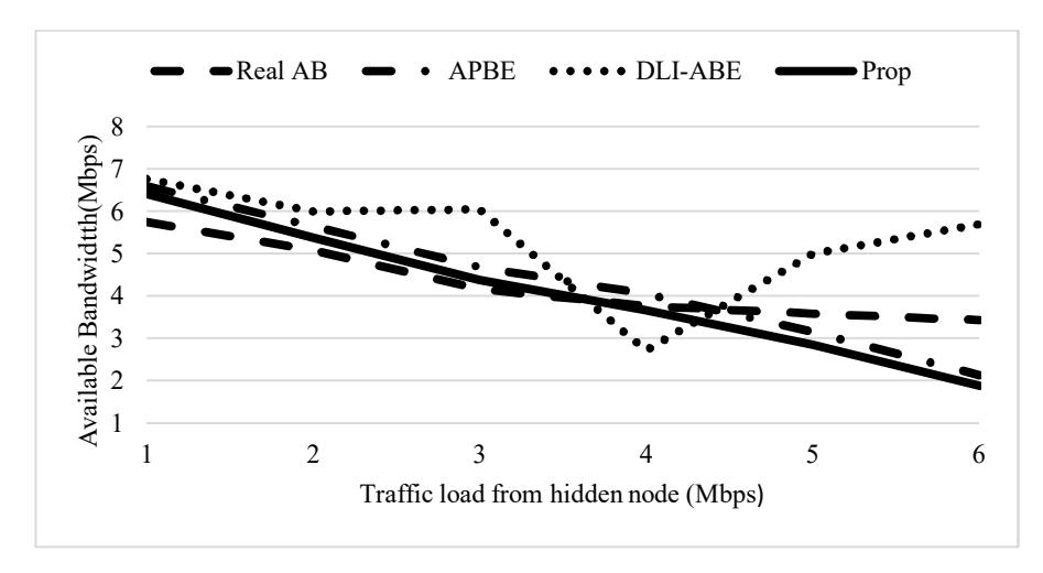
Figure 5 Accuracy comparison of three schemes.
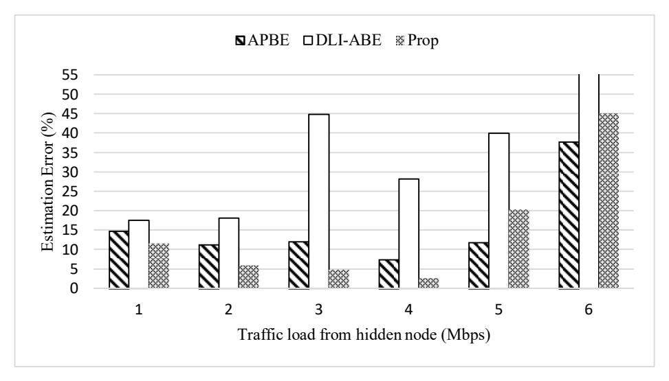
Figure 6 Estimation error comparison of three schemes.
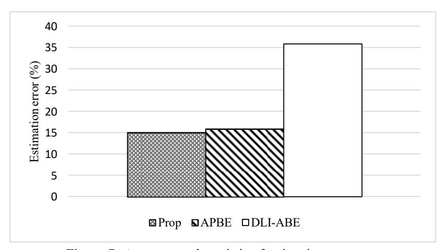
Figure 7 Average result statistic of estimation error rate.
6 Discussion
Available bandwidth estimation in wireless networks is an important function for network resources management and service provisioning that can guarantee QoS of multimedia real-time applications [2]. Several challenges for estimating available bandwidth in wireless networks are collision probability estimation, idle-period synchronization at the sender and receiver nodes, intra-flow contention, and identification of nodes within the carrier sense range [3].
Our proposed scheme was developed based on two existing schemes, DLI-ABE and APBE. DLI-ABE assumes that packet collision probability depends on packet length. In our proposed scheme, the probability of collision between packets is calculated based on average backoff window size (control access to the medium) and number of neighboring nodes (number of neighbor nodes trying to access the same medium). In addition, when compared with APBE, it only considers channel idle time on the sender and receiver nodes but does not take into account the transmission of data packets from other nodes that can affect the state or condition of both the sender and the receiver node. Chaudhari, et al. [3] state that the medium on the sender node must be in free condition, so that the medium can be accessed to transmit data packets. In addition, at the same time, the receiver node must also be in free condition during the time required to transmit whole data packets, in order to avoid collisions. Both of these conditions are provisions to estimate the available bandwidth accurately. Furthermore, the medium condition of a node can be influenced by the flow of data packets originating from other nodes. Based on this, we took into account idle-period synchronization between the sender and receiver nodes to estimate available bandwidth.
7 Conclusion
We have presented a bandwidth estimation approach with involvement of some factors that can affect available bandwidth. These factors are: proportion of transmission waiting time and backoff delay; probability of packet collision; acknowledgment delay; and synchronization channel conditions compared to measurement time. Random transmission waiting time was calculated based on DIFS and average backoff time. Packet collision probability was calculated based on number of nodes and position of those nodes. Delay acknowledgment that acts as a control message was calculated based on acknowledgment frame transmission timeout and SIFS overhead. Node state synchronization was calculated based on a model for idle-period synchronization at the sender and receiver nodes.
Based on our experiment, we found that when hidden nodes generating traffic load consumed approximately 52% of the maximum bandwidth capacity, the proposed scheme could estimate the available bandwidth more accurately compared to the other two schemes. When hidden nodes generating traffic load consumed more than 52% of the maximum bandwidth capacity, the available bandwidth estimated by the proposed scheme was inaccurate compared with that from the APBE scheme. However, the overall result of the estimated available bandwidth generated by our proposed scheme on a wireless network was the most accurate when compared to the other two schemes, estimating available bandwidth 0.9% more accurately when compared to APBE and 21.8% more accurately when compared to DLI-ABE.