
1 Introduction
In general, there are two conditions (or requirements) that limit the execution of a computation, namely: the accuracy of the results and processing time. If the first requirement is used, then the main purpose of the computation design is to maximize the accuracy of the results. Getting more accurate results usually takes longer processing time. With the second requirement, if it is assumed that the accuracy of the desired result stays the same, the challenge is to shorten the execution time. One possible approach to shorten execution time is reducing the number of executed computation units. In [1] and [2] we proposed a new computation strategy to reduce the execution time, named Double Track – Most Significant Operation First (DT-MSOF). This strategy uses the concept of intermediate result, ordering executions based on their level of significance, uses an approximate computing approach, and restricts execution using an interval arithmetic concept.
One popular technique to support the multi-criteria decision-making process is Analytic Hierarchy Process (AHP), developed by Saaty [3]. Three main principles are used in decision-making using AHP, namely: decomposition, comparative assessment, and synthesis of priority values. The purpose of this paper was to implement the DT-MSOF strategy to modify the AHP algorithm so that the number of operations needed to get the right decision will be smaller than needed by conventional AHP algorithms.
The DT-MSOF strategy can be used for computations with the following characteristics:
- 1. The computation has a numerical based calculation and is continued with the decision-making.
- 2. Changes in the order of execution of computational elements do not affect the end result.
- 3. The level of significance (contribution to the final result) of all computational elements can be determined.
- 4. All computational elements are available before the execution starts.
The AHP algorithm fulfills all of the above requirements.
In the following part of this paper, a literature review will be presented concerning the MSBF computational concepts that have been developed into MSOF, approximate computing, interval arithmetic, and generic AHP algorithms. The next chapters contain an explanation of the DT-MSOF strategy and its use in modifying the AHP algorithm into DM-AHP. The fifth section contains simulation scenarios that were used to compare the number of operations that needed to be performed with the use of AHP and DM-AHP to get the same decision. The sixth section contains the results of the simulation and discussion.
2 Literature Review
2.1 From MSBF to MSOF
People usually perform arithmetic operations manually by starting from the rightmost number digit/LSB (least significant bit) and then move to the left / MSB (most significant bit). This method is also used in designing arithmetic operations performed by a computer. Using this approach, the accuracy of the results will increase more sharply at the end of the calculation process. To accelerate the increase of accuracy of the calculation results, operations can be performed starting from the leftmost digit (MSB) and then moving to the right (LSB). Arithmetic calculation using the concept of Most Significant Bit-First (MSBF) was first formulated by Nielsen and Kornerup [4]. This approach has been used in the hardware domain to accelerate the increase of calculation accuracy in arithmetic operations [5], to improve the performance of the Viterbi decoder [6,7] and the variable block size motion estimation processor for H.264/AVC video coding [8]. We used MSBF as an inspiration and tried to expand its use to the scope of operations or computing elements so that computing can be executed in the Most Significant Operation-First (MSOF) order.
By using MSOF, a sequential operation is performed according to the level of its significance (contribution to the final result). Execution of the operations will be carried out in the order starting from the most significant operation. When MSOF is combined with the intermediate-result concept, some operations done at the end will have less impact on the final result than work done at the beginning. To shorten the computing time, these operations that have no significant impact are considered unnecessary and will not be executed. Figure 1 illustrates the progress of the function execution and the accuracy of the result using three different approaches: without using either intermediate result or MSOF; using the intermediate result but without MSOF; and using both intermediate result and MSOF.
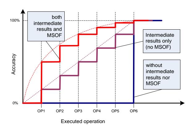
Figure 1 Accuracy versus the number of executed operations using 3 different approaches [1].
2.2 Approximate Computing
In the computation domain, there is a group of programs that contain parts that are not critical. Inaccurate calculations on the uncritical part will not significantly affect the quality of the final result (Quality of Result/QoR) and do
not affect the user's perception of the particular result. For example, Esmaeilzadeh, et al. [9] showed that for 3D ray tracer applications, about 98% of floating-point operations and 91% of data access turned out not to be a critical operations. Some iterative algorithms also have this character. Running a number of calculations with reduced precision, they can still provide a QoR that remains the same [10-12].
The first step in approximate computing is to determine which part of the operation and/or data can be approximated. After it has been determined which part of the application is not sensitive to error and does not have a large effect on the final result, approximation can be done on that particular part. There are some strategies to do the approximation, including changing the precision (bit width) of the input or the intermediate operand to save memory, energy, or other computing resources [12], and limiting iterations done on a recurrent part to reduce computing overhead [13]. How aggressive the approximations can be made is limited by the correctness assurance of the end result of the computation and/or tolerance given by the user, e.g. the approximations performed on the data compression program should not make the decompression results differ from the original data (in the case of lossless compression) or beyond the user's tolerance (in the case of lossy compression).
2.3 Interval Arithmetic and Double-Track Computation
Arithmetic intervals were originally developed by Moore & Yang [14,15] to perform error analysis on automatic computer calculations. Conventional arithmetic defines an operation against operands, each of which is a single number, while an interval arithmetic defines an operation against an interval number. In the interval number system, each number (X) is represented by two values, namely: the lower bound value (xl) and the upper bound value (xu). The interval arithmetic operation is performed on these two values. The two boundary values indicate the range in which the value of the actual operating result lies. The width of the range between two boundary values can also indicate how accurate the calculation results are.
This interval arithmetic concept can be used to determine which operations of a computation do not need to be done while maintaining the user's perception of the computing outcome. Along with the calculation of the original function in each phase, the calculation of the lower bound and upper bound values is also done (that is why we call the method Double-Track Computation). The lower bound and upper bound values will be used in the decision-making process to determine whether execution needs to be continued to the next operation or the execution result is considered sufficient to meet the needs of the user.
2.4 Analytic Hierarchy Process
In order to make decisions based on priorities, the steps that generally need to be performed in the AHP algorithm are as follows [16]:
- 1. Define the problem and specify the type of information needed.
- 2. Arrange the decision hierarchy from the highest level containing the final decision-making goal, the middle level containing the set of criteria (and sub-criteria if any), and the lowest level containing available alternatives.
- 3. Create a pairwise comparison matrix. Each element at a higher level is used to compare elements at the level right below it.
- 4. The priority value obtained from the comparison process is used to give weight to the priority at the level right below it. This process is done for each element. Then, for each element at the bottom level, summation is done to get its global priority value. This weighting and summing process continues until the last priority value at the bottom level is reached.
Several studies have proposed modifications of the AHP algorithm, including prioritizing divergent intangible alternatives [17], improving the consistency ratio of the pairwise comparison matrix [18], contradiction mitigation judgment [19], and modifying the priority vector derivation [20]. The AHP algorithm can also be combined with other methods, including fuzzy set theory, data envelopment analysis, mathematical programming, quality function deployment, simulation, and others [21]. The conventional AHP algorithm, the modified AHP algorithm, and the integration performed on the AHP algorithm generally use the run-to-completion approach.
3 DT-MSOF Strategy
There are three major components in this computational strategy, namely: sorting of computing elements, calculation (execution of computational elements), and decision-making. The relationship between these components is shown in Figure 2. The system requires input in the form of computational functions, data associated with each part of the function, and the criteria required as a basis for decision-making. Each time a decision is needed, the first step is to make an ordering of the computational elements (function and/or data) based on their significance. Calculations are then executed following the order of significance to get an intermediate result. In this strategy, the intermediate result is a combination of a certain value with an uncertain value. The intermediate result is defined as two boundary values, i.e. the lower bound value, and the upper bound value with the following formulation:
1. Upper bound = result from the computations executed so far + maximum value of the unexecuted computations.
2. Lower bound = result from the computations executed so far + minimum value of the unexecuted computations.
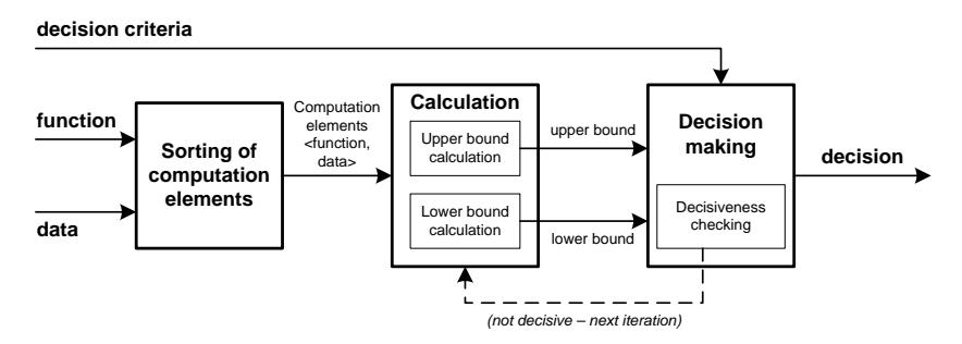
Figure 2 Block diagram of DT-MSOF strategy.
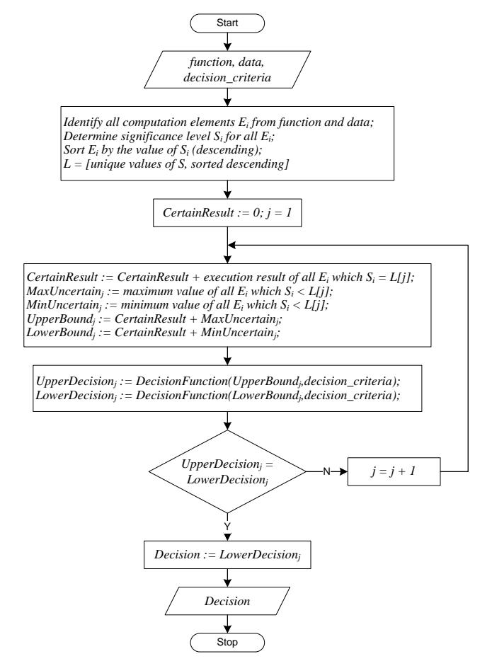
Figure 3 Flowchart of DT-MSOF strategy.
At each iteration, the upper bound value is monotonically non-increasing, while the lower bound value is monotonically non-decreasing. The boundary values are then used for decision-making using the specified criteria. If a decision cannot yet be made (decisive conditions have not yet been reached), then the execution is performed for the computational element at the next level of significance. The cycle of calculation and decision-making continues until a decision can be determined. The high-level flowchart of DT-MSOF strategy is depicted in Figure 3.
4 DM-AHP: the Modification of AHP using DT-MSOF Strategy
By considering the AHP algorithm above, there are several findings:
- 1. AHP uses a run-to-completion strategy (all data and calculations must be done and completed first before making a decision). In certain cases there can be overkill (calculations done beyond the need for decision-making).
- 2. DT-MSOF is proposed to save the number of executed calculations to the limit that is just sufficient to make a correct decision. This is expected to increase efficiency (save processing time and resource use) and increase the productivity of decision support systems because in the same time it will be able to complete more tasks.
There is an opportunity for the following modifications:
- 1. After the step of pairwise comparison against the criteria (and sub-criteria), it turns out that the priority value of each criterion (and sub-criteria) to the objectives also indicates the significance level of each of the criteria (and sub-criteria), which can be exploited by the strategy of Most Significant Operation-First.
- 2. In the decision-making step, there is a process of summing alternative priorities against criteria for each alternative that has the characteristics of increased reward with increased service (IRIS), which can be exploited by the strategy of Double-Track Computation.
Based on the study, modifications were made to the AHP algorithm by incorporating the DT-MSOF strategy into the AHP algorithm. A comparison between the original AHP algorithm and the modified algorithm (referred to as DM-AHP) can be seen in Table 1.
The number of global steps in the DM-AHP algorithm is larger than in conventional AHP. Of the two algorithm variants, we need to pay most attention to the most dominant operation, which is the pairwise comparison between alternatives with criteria (and sub-criteria). From the structure of each algorithm it can be concluded that the number of pairwise comparison
operations that occur in DM-AHP (DM-AHP step 5a) can be smaller than the number of pairwise comparisons that occur in conventional AHP (AHP step 4). This can be explained as follows: in AHP step 4, the comparison is performed on all alternatives for all criteria (and sub-criteria), while in DM-AHP, pairwise comparisons in step 5a are carried out on alternatives and criteria (and subcriteria) iteratively only until conditions are reached that allow decision-making.
Table 1 Comparison between the AHP and DM-AHP algorithms.
| AHP | DM-AHP | ||
|---|---|---|---|
| 1. | Construct the hierarchy | 1. | Construct the hierarchy |
| 2. | Pairwise comparison of the criteria with respect to the | 2. | Pairwise comparison of the criteria with respect to the goal |
| goal | 3. | Check the consistency | |
| 3. 4. | Check the consistency Pairwise comparison of the | 4. | Sort the criteria's priority (descending) //the role of MSOF |
| alternatives with respect to the criteria | 5. | For each criterion (starting from the highest priority) do: | |
| 5. | Making the decision | a. Pairwise comparison of the alternatives with respect to the criteria | |
| b. Calculate the lower bound and the upper bound | |||
| //the role of DT | |||
| c. Check the conclusiveness | |||
| d. If conclusive then make the decision |
The purpose of the DT-MSOF strategy is to accelerate computing while maintaining the quality of the final results. Thus, the final decision produced by the DM-AHP algorithm should be the same as the decision produced by the conventional AHP algorithm.
To calculate the lower bound and upper bound, the following formulas are used:
Lower bound (i) = \[\begin{cases} 0\%, & i = 0 \\ \sum_{n=1}^{i} global \ priority \ of \ alternative(n), & i > 0 \end{cases}\] (1)
Lower bound (i) = \[\begin{cases} 0\%, & i = 0 \\ \sum_{n=1}^{i} global \ priority \ of \ alternative(n), & i > 0 \end{cases}\] (1) \[\text{Upper bound (i)} = \begin{cases} 100\%, & i = 0 \\ 0\%, & i = NC \\ Lower \ Bound(i) + max \ uncertain(i), & i > 0 \end{cases}\]
\[\max uncertain(i) = \sum_{n=i+1}^{NC} global \ priority \ of \ criteria(n)\] (3)
\[NC = number \ of \ criteria\] (4)
There are two additional rules used in the determination whether an operation will continue to be done or not, and used in the examination of the achievement of a decisive condition, namely:
- Rule # 1: Priority values of the (criteria, alternatives) pair whose upper bound value is already lower than the lower bound value of a superior alternative (winner candidate) does not need to be counted again.
- Rule # 2: The decisive condition is obtained when the lower bound value of an alternative is already higher than the upper bound value of all other alternatives.
5 Simulation
To give an example of the use and effectiveness of DM-AHP, a decisionmaking simulation was done with the case of 'family car selection', which is available online at http://en.wikipedia.org/wiki/Analytic_hierarchy_process_– _car_example. The relative importance of the pairwise comparison between criteria and sub-criteria and the pairwise comparison between alternatives for each criterion and sub-criteria is used from the web page. Priority values are recalculated using AHPcalc Excel Template Version 2016.05.04 available at http://bpmsg.com/new-ahp-excel-template-with-multiple-inputs/.
The first step up to the third step of AHP and DM-AHP are the same and at the end of the third step the value of local and global priority to the goal of all criteria and sub-criteria will be obtained. The values were as shown in Table 2.
| Table 2 | Priority value of all criteria and sub-criteria in the 'Family Car | |||||
|---|---|---|---|---|---|---|
| Selection' case. |
| Criteria | Sub-criteria | Local | Global |
|---|---|---|---|
| Cost | 51.00% | ||
| Purchase price | 48.80% | 24.89% | |
| Fuel cost | 25.20% | 12.85% | |
| Maintenance cost | 10.00% | 5.10% | |
| Resale value | 16.10% | 8.21% | |
| Safety | - | 23.40% | 23.40% |
| Style | - | 4.10% | 4.10% |
| Capacity | 21.50% | ||
| Cargo | 16.70% | 3.59% | |
| Passenger | 83.30% | 17.91% |
In order to be able to do a pairwise comparison between alternatives for each criterion (step 4 in AHP and step number 5a in DM-AHP), local priority values are required from all alternatives to the criteria. These values were calculated and obtained as shown in Table 3.
Table 3 Local priority values of all alternatives to criteria and sub-criteria in 'Family Car Selection' case.
| Alternatives | Purchase price | Fuel cost | Mainte-nance cost | Resale value | Safety | Style | Cargo | Passenger |
|---|---|---|---|---|---|---|---|---|
| Accord S | 24.60% | 18.70% | 35.80% | 22.50% | 21.60% | 35.80% | 8.90% | 13.60% |
| Accord H | 2.50% | 21.10% | 31.30% | 9.50% | 21.60% | 35.80% | 8.90% | 13.60% |
| Pilot | 2.50% | 13.20% | 8.40% | 5.50% | 7.50% | 3.90% | 17.00% | 27.30% |
| CR-V | 24.60% | 16.30% | 10.00% | 41.60% | 3.60% | 15.50% | 17.00% | 13.60% |
| Element | 36.60% | 15.10% | 8.80% | 10.50% | 2.20% | 2.30% | 17.00% | 4.50% |
| Odyssey | 9.30% | 15.70% | 5.70% | 10.50% | 43.40% | 6.80% | 31.10% | 27.30% |
The simulation was done by performing several calculations using AHP and DM-AHP. For each simulation scenario, the local priority value of the alternative against the criterion was fixed (using the values listed in Table 3).
6 Results and Discussion
In order to determine the impact on the amount of computing required in decision-making, in addition to using the values in Table 2, the priority criteria and sub-criteria values for the goal were changed. Table 4 contains the global priorities of the criteria and sub-criteria used in 7 simulation scenarios. The values from Table 2 were copied into the column 'scenario 2'. The bottom row of Table 4 contains the standard deviation value of each column.
Table 4 Global priority values of all criteria and sub-criteria used in the simulation.
| Criteria / | scenario | scenario | scenario | scenario | scenario | scenario | scenario |
|---|---|---|---|---|---|---|---|
| sub-criteria | 1 | 2 | 3 | 4 | 5 | 6 | 7 |
| Purchase price | 12.50% | 24.89% | 11.68% | 0.99% | 0.99% | 0.99% | 0.99% |
| Fuel cost | 12.50% | 12.85% | 6.66% | 0.56% | 0.56% | 0.56% | 0.56% |
| Maintenance cost | 12.50% | 5.10% | 30.66% | 7.00% | 5.00% | 2.60% | 2.60% |
| Resale value | 12.50% | 8.21% | 21.81% | 1.00% | 1.00% | 1.85% | 1.00% |
| Safety | 12.50% | 23.40% | 14.60% | 35.00% | 45.00% | 44.90% | 60.00% |
| Style | 12.50% | 4.10% | 5.90% | 10.00% | 10.00% | 4.20% | 4.00% |
| Cargo | 12.50% | 3.59% | 0.86% | 25.00% | 25.00% | 40.41% | 25.00% |
| Passenger | 12.50% | 17.91% | 7.74% | 20.45% | 12.45% | 4.49% | 5.85% |
| STDEV | 0.00% | 8.10% | 9.06% | 12.09% | 14.50% | 17.49% | 19.48% |
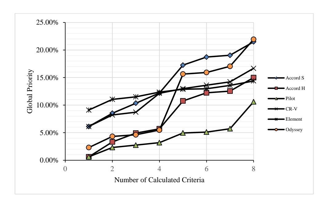
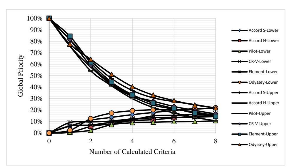
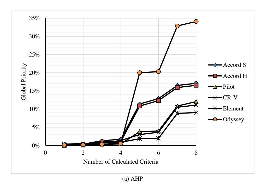
The focus of the simulation observation was the amount of computation that needs to be done in the pairwise comparison process between the alternatives for each criterion until the decision could be made (steps 4 and 5 in the AHP algorithm; step number 5a to 5d in the DM-AHP algorithm). Figure 4 to Figure 6 contain charts showing the difference in the movement of global priority values of each alternative obtained when using the AHP algorithm with those obtained when using the DM-AHP algorithm for scenarios 2, 3, and 6.
(a) AHP
(b) DM-AHP
Figure 4 The movement of the global priority value of each alternative for scenario 2: (a) using AHP and (b) using DM-AHP.
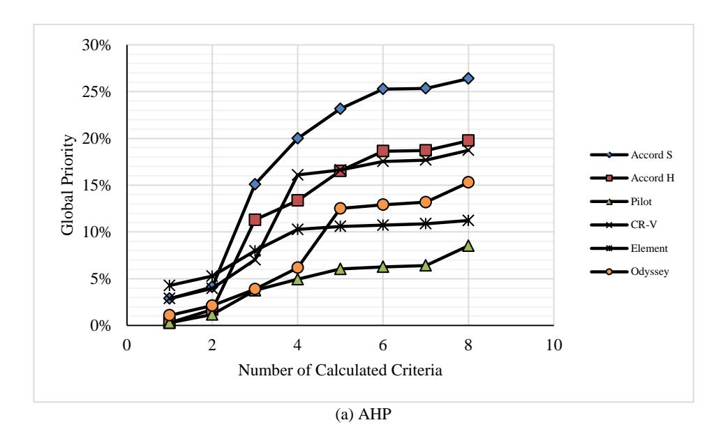
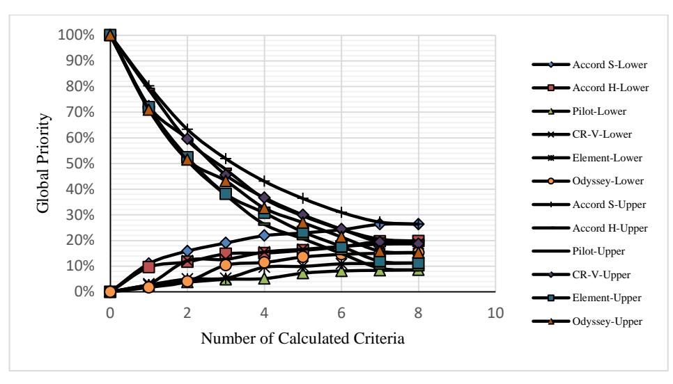
Figure 5 The movement of the global priority value of each alternative for scenario 3: (a) using AHP and (b) using DM-AHP.
(b) DM-AHP
0% 10% 20% 30% 40% 50% 60% 70% 80% 90% 100% 0 2 4 6 8 Global Priority Number of Calculated Criteria Accord S-Lower Accord H-Lower Pilot-Lower CR-V-Lower Element-Lower Odyssey-Lower Accord S-Upper Accord H-Upper Pilot-Upper CR-V-Upper Element-Upper Odyssey-Upper
(b) DM-AHP
Figure 6 The movement of the global priority value of each alternative for scenario 6: (a) using AHP and (b) using DM-AHP.
Using the AHP algorithm, it is necessary to first calculate the global priority value for all combinations of alternative and criteria (in this case 6 alternatives x 8 criteria = 48 calculations) before the final decision is made (the alternative with the highest priority value at the end of the computation). Although the winner alternatives in Figures 5(a) and Figure 6(a) had the highest priority values – from the first criteria – and persisted to the end, they could not serve as a basis for stopping the computation and making decisions right away at that moment. The phenomenon shown in Figure 4(a) is an example of falsification. An alternative that has a high priority value on some of the first criteria is not the final winner since its value is not the highest when the last criterion is evaluated.
The DM-AHP algorithm can avoid such problems because the use of lower bound and upper bound values and two additional rules as listed in Section 4 can reduce the number of calculations that need to be made to make decisions. The use of DM-AHP in scenario 2 (Figure 4(b)) could save the calculation of 5 operations (reduction of 10.42% when compared to the total calculation required by AHP). The explanation is as follows:
- 1. In criterion 6: Pilot's upper bound value (Pilot-Upper) has already been executed below the Odyssey's lower bound value (Odyssey-Lower)
- 2. In criterion 7:
- a. The Pilot alternative no longer needs to be calculated (according to additional rule number 1), resulting in a reduction of 2 operations (1 alternative x 2 criteria)
- b. The upper bound of CR-V (CR-V-Upper), the upper bound of Accord H (Accord H-Upper), and the upper bound of Element (Element-Upper) are below the lower boundary of Accord S (Accord S-Lower).
- c. The possible winners left are only 2 alternatives, namely: Accord S and Odyssey (1/3 of the overall alternatives).
3. In criterion 8:
- a. The CR-V, Accord H, and Element alternatives do not need to be calculated (according to additional rule number 1), resulting in a reduction of 3 operations (3 alternatives x 1 criteria).
- b. The winner is obtained, namely the Odyssey (according to general rules of AHP and additional rule number 2)
The use of DM-AHP in scenario 3 (Figure 5 (b)) can save the calculation of 10 operations (reduction of 20.83%) with the following explanation:
- 4. In criterion 5: the Pilot-Upper value is already below the Accord S-Lower value.
- 5. In criterion 6:
- a. The Pilot alternative no longer needs to be calculated (according to additional rule number 1), resulting in a reduction of 3 operations (1 alternative x 3 criteria).
- b. The Odyssey-Upper and Element-Upper values are already below the Accord S-Lower value.
6. In criterion 7:
- a. The Odyssey and Element alternatives no longer need to be calculated (according to additional rule number 1), resulting in a reduction of 4 operations (2 alternatives x 2 criteria).
- b. The winner is obtained, namely the Accord S (according to additional rule number 2)
- c. Criterion 8 does not need to be evaluated, resulting in a reduction of 3 operations (3 alternatives x 1 criteria).
Using DM-AHP in scenario 6 (Figure 6 (b)) can save the calculation of a total of 36 operations (reduction of 75.00%) with the following explanation:
7. In criterion 2:
- a. The Odyssey-Lower value is above all other upper bound values
- b. A winner is obtained, namely the Odyssey (according to additional rule number 2)
- c. Criteria 3 and so forth do not need to be evaluated, resulting in a reduction of 36 operations (6 alternatives x 6 criteria).
The scenarios listed in Table 4 are designed in such a way as to obtain the diversity of the distribution of priority values from the criteria. The distribution of priority values is represented by the value of standard deviation. Scenario 1 has standard deviation = 0%, which means all criteria have the same priority value (i.e. the significance weight is the same in decision-making). This standard deviation value was larger in the subsequent scenarios, up to 19.48% in scenario 7.
The simulation results show that this standard deviation value influences the percentage of reduced operations, as seen in Table 5. Figure 7 shows that the greater the standard deviation value (which indicates a greater difference in significance between criteria), the greater the percentage of operations that can be reduced to reach a correct decision using DM-AHP.
This phenomenon can be explained as follows. If the priority value among the criteria is different, then MSOF is able to determine the order of calculation execution starting from the highest priority (because it is considered the most significant). The greater the priority value of a criterion, the greater its contribution to the decision-making result. If the distribution of priority values for all criteria is wider (indicated by an increased standard deviation value), then the criterion executed first will have an increasingly dominant contribution to the final decision. The criteria at the end of the execution sequence will not have a significant impact so they can be ignored in making the decision (the same decision as when all criteria were involved). Double track computing plays a role in determining when a computation should proceed to the next criteria or be considered sufficient to make a decision.
Table 5 Number of operations in AHP and DM-AHP for each standard deviation value.
| Standard deviation of priority criteria | |||||||||||
|---|---|---|---|---|---|---|---|---|---|---|---|
| 0% | 8,10% | 9,06% | 12,09% | 14,50% | 17,49% | 19,48% | |||||
| Number of comparison using AHP | 48 | 48 | 48 | 48 | 48 | 48 | 48 | ||||
| Number of comparison using MD AHP | 47 | 43 | 38 | 24 | 21 | 12 | 12 | ||||
| Number of reduced operation | 1 | 5 | 10 | 24 | 27 | 36 | 36 | ||||
| Percentage of reduced operation | 2,08% | 10,42% | 20,83% | 50,00% | 56,25% | 75,00% | 75,00% | ||||
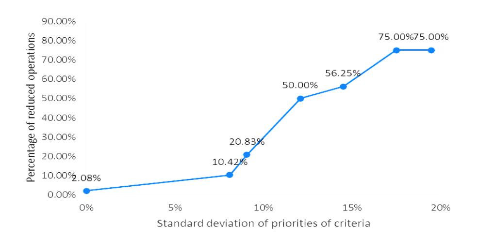
Figure 7 The effect of standard deviation of criteria priorities on the percentage of reduced operations in the use of DM-AHP.
7 Conclusion
This paper presented the Double-Track Most Significant Operation-First (DT-MSOF) strategy and its application to modify the Analytic Hierarchy Process (AHP) algorithm. A simulation was performed to compare the number of pairwise comparison operations required by the conventional AHP algorithm to those required by the DM-AHP algorithm. The variable that was modified in each scenario was the global priority value of the criteria and sub-criteria. Changes were made so that the standard deviations of priority values were approximately 0.00%, 8%, 9%, 12%, 14.5%, 17.5%, and 19.5%. The simulation results showed that the percentage of the reduction in the number of pairwise comparison operations in the DM-AHP algorithm compared with the conventional AHP algorithm was 2.08%, 10.42%, 20.83%, 50%, 56.25%, 75%, and 75% respectively. The new DM-AHP algorithm was proven to be effective in reducing the number of operations that need to be done to get the same result (decision) as obtained by conventional AHP.
The more uneven the distribution of priority values (the larger the standard deviation), the more operations can be reduced (do not need to be executed). This suggests that the DT-MSOF strategy is more suitable for use in problem areas that have an uneven distribution of operation (or computational elements) significance.
8 Future Work
In order to accelerate the achievement of a decisive condition, it is possible to do further investigation on the formulation of the upper bound to get a lower value, i.e. the uncertain part is not the maximum value, and the possibility of prediction of lower and upper bound values for criteria that have not been calculated (e.g. by extrapolation, statistics-based, or other techniques).
Acknowledgment
This work was supported by Institut Teknologi Bandung through grant P3MI 2017.