
1 Introduction
The metal production industry is the backbone of India's economy. In order to produce more value-added products it is necessary to take product quality control into consideration. Predominant occurrence of defects in metal objects during manufacture leads to losses. To improve the metal production process it is necessary to use advanced technologies and practices, one of which is applying automated defect detection and characterization on metal objects. A defect is a flaw in a product or a part of a product that fails to meet the minimum applicable acceptance specifications, benchmarks and standards.
During manufacture – i.e. fabrication, assembly, and servicing – some materials may incur defects. Some of these may be inherent to the nature of the material. Defects can be classified into two types, i.e. surface defects and subsurface defects. Surface defects are defects that are visible in the upper layer of the object. Subsurface defects reside in the inside layer of the object. Cracks, spots, edges, pinholes and scratches are the most commonly occurring types of defects in metal objects. Defect detection on metal objects can be done using various NDE techniques. Magnetic particle testing (MPT), radiographic testing, ultrasonic testing, visual testing, thermographic testing, and eddy current testing are some examples of NDE techniques. Thermographic inspection is used for NDE of parts and materials by analyzing thermal patterns on the object's surface [1,2].
Thermography refers to all available techniques in thermographic inspection, irrespective of the phenomena used for monitoring the thermal change rate. Various thermographic inspection methods are available for defect detection, among others pulse phased thermography (PPT), thermal signal reconstruction, partial least square thermography, principal component thermography, higher order statistics. Infrared thermography (IRT) is one of the most popular and advanced NDE technologies. It has gained wide application due to its capability of covering a large area in a small amount of time. It delivers a complete noncontact field image. IRT is considered safe because it does not involve harmful or hazardous radiation in contrast to radiography for instance.
Due to the increased prominence of defect detection and characterization, some new techniques have been introduced, such as lock-in thermography (LT) and pulse thermography (PT).
In LT, a modulated light source is used to continuously heat up the material, which will result in thermal waves on the surface of the material. This thermal wave pattern is continuously monitored via thermal imaging. For each pixel, a Fourier analysis is carried out in order to obtain amplitude and phase images.
PT is an advanced NDE technique that can be used in defect detection. In PT, the surface of the specimen or testing material is excited by a short heat pulse and the temperature response of the material is monitored using infrared cameras. The temperature response pattern will differ in a defective area compared to a non-defective area and thus the thermal response provides information about material defects.
Automation plays an important role in the modernization of production lines and it also enables to meet the standards of the global market [3]. This paper presents a novel automated system for defect detection and characterization of metal objects using pulse thermography images and various image processing techniques.
2 Related Work
This section discusses image processing techniques for image preprocessing, defect detection and characterization. Image preprocessing is an important phase before performing any operations on the images because most of the images contain noise, blurring and imperfections related to brightness and the geomagnetic values of the pixels.
Adatrao, et al. [4] presents an overview and analysis of two filters and some image segmentation techniques, specifically comparing median filtering and Wiener filtering. They investigated image segmentation methods such as Prewitt, Sobel, Roberts, LoG (Laplacian or Gaussian), basic global and Otsu's global thresholding, and canny edge detection. Finally, they carried out a qualitative comparison of the results by visual inspection. Castanedo, et al. [5] discuss various techniques and methods, such as radial distortion correction, noise smoothing, pixel enhancement, pulse phased thermography (PPT) and principle component analysis (PCA), which they used to carry out data analysis. They also present various factors that cause quality degradation in an image, such as fixed pattern noise, vignetting, radial restoration and finding dead pixels. Pulse thermography images are affected by quality degradation with respect to time. Shepard, et al. [6] illustrated a novel thermal signal modernization technique to classify longitudinal non-uniform and chronological noise constituents present in an image. This classification helps to reduce chronological and non-uniform image noise. A significant decrease in the data structure size allows simultaneous processing of multiple data sequences and analysis. The technique works well with small datasets but is only moderately applicable to larger datasets. Forstner [7] discusses image preprocessing for feature extraction in color, digital intensity and range images. He used a signal dependent noise variance function to remove noise from the image.
Defects fall into various categories. After successful detection it is necessary to classify them based on several factors, for example type and size. Aarthi, et al. [8] implemented a novel method for a detailed analysis of surface defects using the wavelet transform. It uses a subband coding algorithm for feature extraction. Statistical analysis is carried out based on mean, standard deviation, variance and skewness of the acquired image. They conducted a comparative study on the Daubechies and Haar wavelets. The quality and reliability of the tests carried out using the wavelet transform were substantially affected by false signals and noise.
IRT is an advanced NDE technology that has gained renown due to its capability to cover a large area in a small amount of time. Milovanovi, et al. [9] present a review on active infrared thermography (IR) for defect detection. They give a brief summary of active IR, various post-processing methods and key equipment required for thermogram analysis. Their method worked well with the experimental dataset. Additional research could be done to prove the feasibility of the system in real-time defect detection. Zheng, et al. [10] implemented an automatic defect detection application by using segmentation techniques on pulsed thermographic images. Defect detection was done in an experiment by making use of the Laplacian eigenmap algorithm and a carbonfiber-reinforced plastic (CFRP) sample. The results were used to prove the feasibility of the algorithm. The paper focused more on segmentation. Sun [11] demonstrated the use of four defect detection methods, i.e. the logarithmic peak second derivative method, the peak temperature constant method, the peak temperature contestant slope method and least square fitting. It was proved that the four methods provide good accuracy and converge to the theoretical solution under ideal conditions. The methods also detected defects accurately with a significant 3D conduction effect. Almond, et al. [12] implemented a Wiener-Hopf technique for investigating thermal edge effects on minute imperfections. However, the smallest size of the defects it can successfully detect is not mentioned. The technique fails when the defect area is overlapped by intersecting edges.
The method proposed by Saintey, et al. [13] utilizes a mathematical finite modification technique to minimize imperfect sizing issues. They also examined severity, size, penetration and material properties. This method evidences a strong dependency on the full width at half maximum (FWHM) measurements for severity, diameter, crack depth, diameter and the material's thermal properties. The system can measure size only for these properties. Wysocka, et al. [14] implemented a method to measure the size and depth of synthetic defects with rectangular and square cross sections using pulsated IR thermography. The designed system gives numerical data of the metal surface defects based on transfer functions. The method worked well with the experimental synthetic defects, but could be further improved to cope with realtime detection. The paper by Sharath, et al. [1] presents a methodical study to evaluate the accuracy of several PT techniques for defect depth and size investigation of a 316 L stainless steel sheet with synthetic defects. Good correlation was obtained between the experimental and the simulated results. For depth quantification, the logarithmic first derivative is applied. A software application called Thermo Calc 6L is used for theoretical modeling. The system is able to identify and characterize only a limited number of defects.
Some gaps and issues can be identified with the existing works. In the above papers the size of the defects that can be detected is restricted, i.e. most of the techniques fail if the size of the defect is too small and in most of the works size is not considered at all. Diffusion is one of the most important challenges to be considered in thermography. Over time, thermal power leads to diffusion. As a result defects are not properly visible and the shape of the defect is also affected. This needs to be addressed properly. Before proceeding to measure the size of the defect it is necessary to find its boundaries. In this scenario, the shape of the defect is gradually affected by diffusion: each shape of the defect will slightly vary over time, so it is difficult to accurately detect the edges of the defect. Hence, defect characterization is one of the key factors to be considered in this area of pulse thermography.
3 Proposed Methodology
The aim of this study was the design and development of an automated system for metal defect detection and characterization using PT images and various image processing techniques. Here, image acquisition was done using an experimental pulse thermography setup. Each image in the image sequence is different with respect to time. In the present work the image dataset was obtained from the Indira Gandhi Center for Atomic Research (IGCAR).
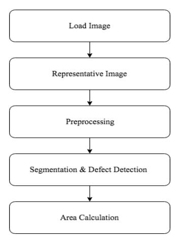
Figure 1 Block diagram of the proposed methodology.
The proposed methodology is divided into a set of subsections, as shown in Figure 1. The first step is the acquisition of images from the object using the PT imaging setup. The captured image dataset is imported into a Matlab host from the IR camera. In the second step, a representative image is obtained from among 250 captured images. Noise present in the representative image is removed by applying a 2-dimensional median filter. Further, a 2-dimensional Wiener filter is applied on the median result. Once the preprocessing is done, the preprocessed images are segmented using the moving window technique. Thresholding, morphological and binarization operations are applied on the defected region to perform sizing. Finally, defect size information on each defect is displayed to the user. The proposed system uses the below defect sizing algorithm.
3.1 Algorithm for Defect Sizing
Input: Pulse thermography images
Output: Defect size
1. Load image dataset consisting of a pulse thermographic image sequence of N images with respect to time t.
T(A, B, t)
where A, B = size of the input images and t is time.
2. Regression by applying the logarithemic polynomial with degree n.
\[ln(\Delta T(A, B, t)) = Img_0(A, B) + Img_2(A, B) + ... + Img_n(A, B)\] where Img0, Img1,……, Imgn is the sequence of images in the dataset. The polynomial co-efficients of (n + 1) images are obtained. A representative image from the (n + 1) polynomial co-efficient images is obtained by polynomial curve fitting.
- 3. Preprocessing of the representative image is obtained using a 2-dimensional median filter and a 2-dimensional Wiener filter.
- 4. Image segmentation and defect detection.
- 5. Calculate defect size in mm.
The information in the pulse thermography dataset is slightly different for each image since they are captured at different time stamps and the experimental sample will be affected by thermal diffusion. Selecting a suitable representative image from the dataset consisting of 250 images is considered a key objective, because processing the complete dataset for each defect is too time-consuming and is not an advisable method for pulse thermography images. A temperature vs time sequence analysis is carried out on the inspection sample. A representative image for further processing is identified. The algorithm processes the complete dataset and finds the most suitable image as the representative image based on polynomial curve fitting. The thermographic image sequence consisting of N images with respect to time t is loaded into the system. This can be represented in Eq. (1) as follows:
\[\Delta T(A, B, t) \tag{1}\] where A, B = the size of the input image and t is time. Regression is done by applying a logarithmic polynomial with degree n as given by Eq. (2):
\[ln(\Delta T(A,B,t)) = Img_0(A,B) + Img_2(A,B) + ... + Img_n(A,B)\] (2)
where Img0, Img1, … Imgn is the sequence of images in the dataset. The firstorder logarithmic deviation is given by Eq. (3):
\[\delta \text{Log}(\Delta T(A,B,t)) / \delta \text{Log}(t)\] (3)
The second-order logarithmic deviation is given by Eq. (4):
\[\delta 2 \left( \text{Log}(\Delta T(A,B,t)) \right) / \delta(\text{Log}(t)) 2 \tag{4}\]
The polynomial co-efficients of (n + 1) images are obtained. A representative image from the (n + 1) polynomial co-efficient images is obtained by polynomial curve fitting.
Preprocessing is done to improve the image by reducing distortion and imperfections, which is necessary for the further processing because in the proposed system the images are affected by noise and blurriness. A 2 dimensional median filter is applied at the first level. This helps smoothing noise. A Wiener filter is then applied to the resultant median image with a window length of 4*4. This reduces the mean square error and helps smoothing noise. It can be articulated in Eq. (5) as follows:
\[W(x_1,x_2) = H^*(x_1,x_2) S_{xx}(x_1,x_2) / |H(x_1,x_2)| 2 S_{xx}(x_1,x_2) + S_{nn}(x_1,x_2)\](5)
where Sxx (x1,x2) and Snn(x1,x2) are the actual spectra and noise spectra respectively. The blurring filter can be represented by H (x1, x2). There are two separate parts in the Wiener filter, a noise smoothing part and the inverse filtering part. The main focus is the noise filtering part.
After pre-processing, the moving window concept is used to segment the image. In the moving window technique, a box or 'slide' is placed around the region of interest and classified based on whether the image contains an object or not. A moving window of 42 pixels for both the column and the row of the image is created. The region within the window is assigned a value 1 (one) and the rest of the region is assigned a value 0 (zero). The moving window technique used in the proposed system is expressed in the following algorithm:
3.2 Algorithm for Moving Window
1. Initialize window size P*Q, where P is the length and Q is the width, both fixed to 42 pixels in the present work.
Image M = i………n where M (i) is a particular image in the dataset.
- 2. The window can be defined with two parameters: start and end.
- 3. Window (k) = [start, end] where start indicates the starting pixel of the image; the region except 42 pixels from the start will be masked. End is the ending pixel.
4. While (obj < 5 || obj > 5)
        {
        ++ M;
        }
if the object detected in the image is smaller or larger than 5 defects, then move to the next image.
5. Once the defects have been detected successfully in the first window move to the next window.
start = end
end = end + 1
Once the defective artifacts have been detected successfully, thresholding is applied with a threshold value of 0.68. As a result, the region of interest will become white and rest of the window black. Morphological operations are applied to the resultant image to increase the efficiency of thresholding. The structuring element is taken as a square with dimensions 4*4. Binarization is done in the next step, because after thresholding and morphological operations some zero pixels (black spots) may still exist in the defective artifacts. Since the image is already in grayscale, binarization applies global thresholding. The pixel value of thresholding changes for every strip. The morphological operation dilation is applied with as structural element a square with dimensions 5*5. When the holes or black pixels in the defective artifacts have been converted to white pixels, each independent connected component is identified (in the experimental dataset this was 5) and the number of connected components in each independent component is identified. The maximum number of unconnected components in the image is considered the total number of defects.
Once, the region has been found, sizing of the defect is carried out. The size is primarily obtained by examining the white pixels present within each defect. Since the only way to measure the size of an image is by using pixels, it is necessary to convert the pixels to mm. The initial size will be in the form of a number of pixels, which is later converted to mm using a correction factor. To convert from pixels to mm, consider the following logic. Let's consider A as a quantity (here A refers to pixels) and X is the required dimension (refers to mm). Consider that A is directly proportional to X as in Eq. (6):
\[A = X \tag{6}\]
Let's consider K as the correction factor. By using Eq. (9), the defect area is calculated and it is derived as follows:
\[A = K * X \tag{7}\]
\[X = A/K \tag{8}\]
\[A^* (1/K) = X \tag{9}\]
4 Results and Discussions
This section explains the details about experimental PT setup, the dataset used in the present work, the graphical user interface and the results of the proposed system. A performance analysis of the system is also discussed in this section.
4.1 Experimental Setup
The sample used in the experiment was an AISI 316L stainless steel plate. The dimensions of the plate were 150*100*3.54 mm. Square-shaped defects were created manually in one side of the plate, as shown in Figure 2. Each defect varied in depth and size. In this sample, defects with a depth of 0.4, 1.13, 1.78, 2.48, 3.17, 3.36 mm respectively were drilled. The size of each square defect was 10, 8, 6, 4, 2 mm respectively. The defects were drilled using an electrical discharge machine (EDM). In the following, all sizes will be in mm (see Figure 2).
To capture an image of the AISI 316L stainless steel plate, a CEDIP Silver-420 infrared camera was used. The AISI 316L stainless steel plate is shown in Figure 4. The camera had a focal plane array with 320 × 250 pixels and an Indium Antimonide (InSb) detector with a Stirling cooling system with a maximum achievable temperature resolution of 25 mK. It detects infrared radiation in the 3-5 µm region and has a maximum frame rate of 176 Hz. For the PT experiment, 2 xenon flash lamps with a power of 1600 W each were used. The flash duration was less than 2 ms. The experiment was carried out in reflection mode.
Stainless steel has a lower emissivity (~0.7), which reduces the emission capacity of the material. To improve the emissivity, a uniform thin coat of black paint was applied to one surface. The camera was kept at a distance of 35 cm from the object while the distance between the lamp and the object was 30 cm. A short pulse of duration 2 ms at 1600 W was injected into the surface of the sample, while the images were acquired at a frame rate of 100 Hz for 2 seconds. A CEDIP silver infrared camera with flash lamp ALTAIR software was used for acquiring the image, as shown in Figure 3. Figure 4 illustrates the experimental setup. The proposed system is represented by the user interface
shown in Figure 5. It has a number of buttons, i.e. Load Dataset, Representative Image, Detect Defect and Sizing. Each button performs the corresponding function. Upon clicking the Load Dataset button a pop-up window appears to select a dataset. The dataset is converted to .mat format and uploaded. The Represtative Image button initializes the variables, processes the complete dataset, analyzes the diffusion pattern segmentation, and executes defect detection and sizing.
Figure 2 AISI 316 L SS plate front surface with defects.
Figure 3 CEDIP silver infrared camera with flash lamps.
Figure 4 Experimental setup.
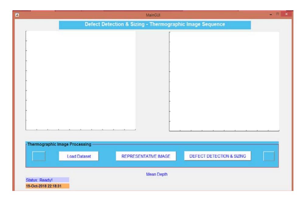
Figure 5 Graphical user interface.
4.2 Dataset
The dataset used for the implementation was constructed based on real sample images obtained from the pulse thermography experimental setup. In the proposed system an image sequence of 250 images is used. All images in the sequence are different from each other because they are taken at a set time interval while the sample is being affected by thermal diffusion.
Size of complete image sequence 3.23 MB, size of individual image 13.7 KB, dimensions: 320*256 320 pixels, width and 256 pixels height 96, dpi horizontal resolution and 96 dpi vertical resolution.
4.3 Performance Analysis
A performance analysis was conducted as a quantitative approach for evaluating the proposed system. The performance of the proposed model was analyzed based on the filtering results, the total number of defects found with depths of 0.4, 1.13, 1.78, 2.48, respectively, and the total time taken by the system.
4.3.1 Defect Detection
In this phase, the performance of the system is analyzed using the relative error as given in Eq. (10). Table 1 gives the relative error of the 5 defects in the metal sheet with 4 different depths. Columns 2 and 5 contain the original defect sizes of the defects. Columns 3 and 6 show the defect sizes obtained from the proposed system. The relative error percentage is shown in the 4<sup>th</sup> and 7<sup>th</sup> columns. The relative error is calculated for all defects using Eq. (10):
Relative error = \[A-D\] (10)
where A is the area obtained from the proposed system and D is the experimental area value. The relative error percentage is given by:
Relative error \[\% = ((A-D) / A) * 100\] (11)
Table 1 shows the defect sizes obtained by the proposed method and the results obtained using the FWHM method [10] for similar experimental data and defect sizes. The proposed method shows an exponential increase in defect size compared to the method proposed by Almond et al.
Table 1 Results obtained using proposed method and FWHM.
| Proposed Method | FWHM | ||||||
|---|---|---|---|---|---|---|---|
| Defects depth | Original defect size | Size obtained from proposed method | Relative error % | Defects depth | Original defect size | Size obtained from proposed method | Relative error % |
| Defects with depth 0.4 mm | 10 | 10.50682 | 5.06817 | Defects with depth 0.4 mm | 9.99 | 9.3 | 10 |
| 8 | 7.02041 | 12.24487 | |||||
| 6 | 4.62871 | 22.85482 | NA | NA | NA | ||
| 4 | 2.61778 | 34.5555 | |||||
| 2 | 1.42788 | 28.606 | |||||
| Defects | 10 | 10.16175 | 1.61745 | Defects with depth 1.13 mm | 9.94 | 9.93 | 0.1 |
| with | 8 | 8.03183 | 0.39782 | NA | NA | NA | |
| depth 1.13 mm | 6 | 4.43833 | 26.02788 | ||||
| 4 | 2.64158 | 33.96055 | |||||
| 2 | 0.76154 | 61.9232 | |||||
| Defects | 10 | 10.19744 | 1.97443 | Defects with depth 1.78 mm | 9.9 | 10.37 | 4.7 |
| with | 8 | 8.35309 | 4.41373 | ||||
| depth 1.78 mm | 6 | 5.71152 | 4.808 | NA | NA | NA | |
| 4 | 3.17703 | 20.57417 | |||||
| 2 | NA | NA | |||||
| Defects with depth 2.48 mm | 10 | 9.65008 | 3.49911 | Defects with depth | NA | NA | NA |
| 8 | 7.99613 | 0.0484 | |||||
| 6 | 6.61584 | 10.26406 | |||||
| 4 | 3.96236 | 0.94082 | 2.48 | ||||
| 2 | NA | NA | mm | ||||
4.3.2 Number of Defects
Similar data investigations have been done with prominent thermographic NDE methods, i.e. HOS [11], PCT [13,14] and PPT [14]. Figures 6 shows the results obtained by the proposed method. The proposed method was able to obtain a huge improvement in defect detection. The performance was also measured based on the number of defects detected in each strip. Here, the defect in each strip was different from the other ones with respect to their depth. Table 2 illustrates this for the first 4 strips.
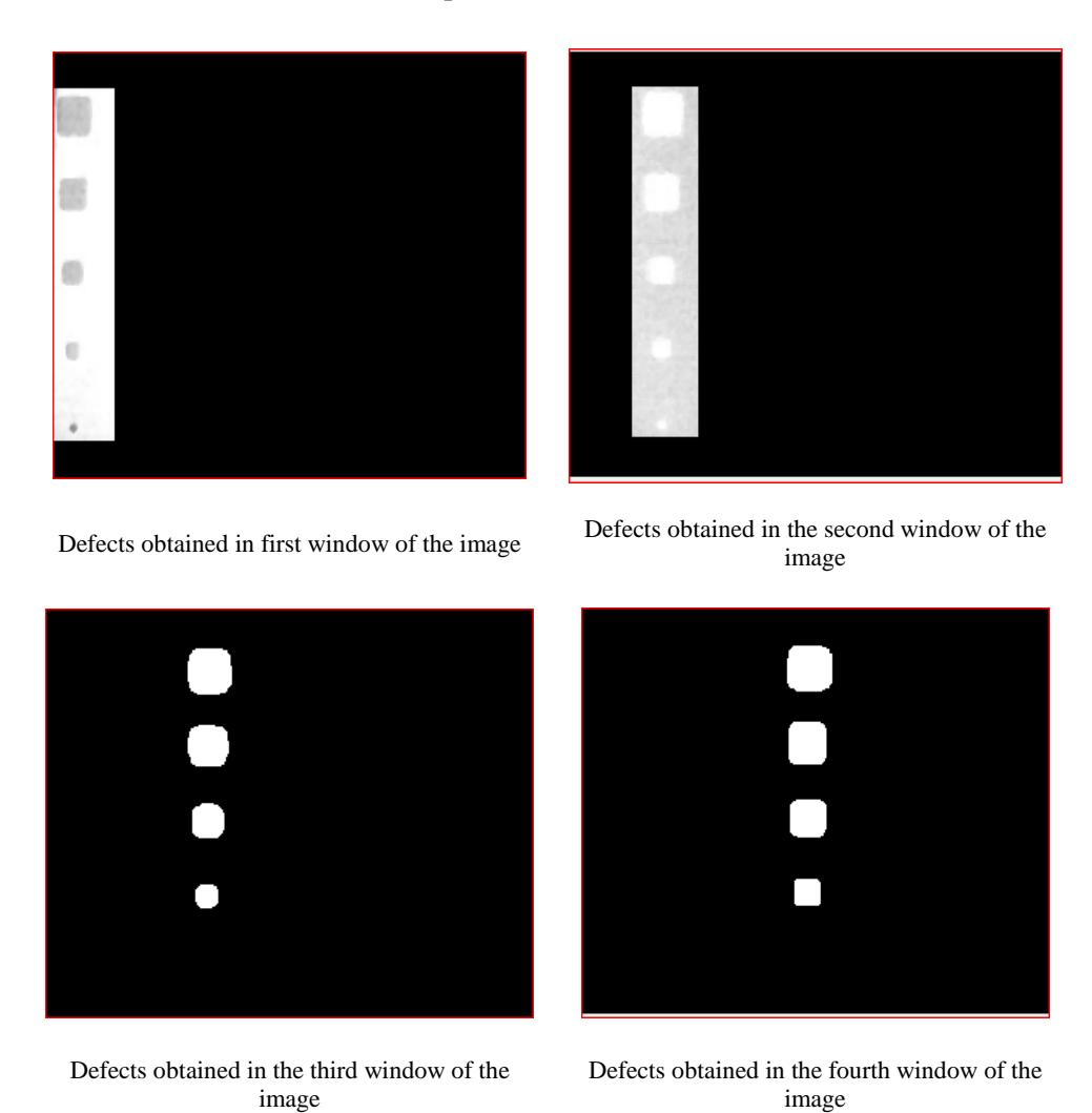
Figure 6 Results obtained by the proposed method. Defect depths of 0.4, 1.13, 1.78 and 2.48 mm respectively were detected.
| Strip Number | Experimental number of defects | Defect count obtained by the proposed system | |
|---|---|---|---|
| Defects with depth 3.36 mm | 5 | 5 | |
| Defects with depth 3.17 mm | 5 | 5 | |
| Defects with depth 2.48 mm | 5 | 4 | |
Table 2 Number of defects detected.
4.3.3 Efficiency of the System
The total time taken for defect characterization was calculated by summing the image loading time, the time required for identifying a representative image, segmentation and defect detection time, and area calculation time. The total time taken by the proposed system for defect sizing was about 7 to 8 minutes. Figure 7 illustrates the defect distribution pattern in the sample after processing the 250 images in the dataset.
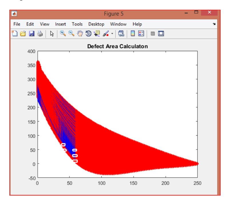
Figure 7 Defect distribution pattern.
5 Conclusion and Future Work
This paper proposed a system for automatic defect detection and characterization in an AISI 316 L stainless steel sheet using pulse thermography images and various image processing algorithms and mathematical tools. The proposed method was applied to 250 images of the sample taken at different time stamps. The method uses a 2-dimensional median filter and a Wiener filter for noise and distortion removal. The moving window concept is used for image segmentation and defect detection. Morphological operations are applied for area detection. The area is calculated by converting pixels into mm using a correction factor. The proposed method can detect defects in a structural material and measures their sizes. The process is automatic and hence can help in effective and efficient characterization of defects in the production of metal objects. Automated defect detection and characterization is an important step to increase production in metal fabrication industries.
Improvements of the defect detection and sizing system to be incorporated in a future work are the following:
- 1. Finding a suitable representative image causes a large amount of delay in the proposed system. Hence, it is necessary to find a technique to overcome this problem.
- 2. The proposed method has successfully detected defects with depth 3.36, 3.17, 2.48, 1.78 respectively in the experimental sample, which is actually a good improvement compared to previous works. This can be further improved to find all defects.
- 3. When the moving window overlaps a defect, the area calculation will give improper results. The method needs to be improved to overcome this drawback.