
1 Introduction
The demand for fast and reliable operations in any organization or business has never been greater, especially in manufacturing, logistics, transportation and various other industries. With the rising costs of operations and management, all businesses are struggling to keep their expenditures low. The greatest potential area for cost saving is manpower administration, through which most organizations pursue approaches that can reduce resource wastage and optimize workforce utilization. This solution is hardly new; [1] presents an optimization software solution for crew rostering to a prominent airline company, which resulted in annual savings of more than USD 20 million. In most organizations, having the ideal amount of manpower is critical as it does not only reduce cost, but also enhances effectiveness and decreases bureaucracy. Therefore, sizable spending by organizations on a viable system for scheduling and rostering is justified and even indispensable as it provides a forecast of the optimal amount of manpower needed. Designing schedules with multiple shifts entails numerous challenges; it is governed by a set of rules or operation constraints that induce complexity in generating an optimum schedule. In an ideal world, a schedule is created using shifts with just the right amount of manpower required. The manpower will be fully utilized during shifts to avoid resource wastage such as idling caused by absence on a job that requires to be completed within a particular period.
Most organizations today still rely on manual shift scheduling, including the organization where we retrieved our data from, namely an airline company based in Kuala Lumpur International Airport. The airline wastes a lot of time and personnel resources just for planning schedules and assigning shifts. In addition, unplanned changes in the airline's daily operation cause chaos in the company and its stakeholders as schedules cannot be re-scheduled promptly. This forced the airline to increase their support staff whose task is only to be standby and take up additional jobs, which results in additional costs. The airline currently spends approximately USD 267 per person a month solely for overtime pay. This cost represents a waste of USD 40,000 per month, or USD 480,000 per year for one department consisting of 150 people.
Shift scheduling algorithms aim to address the challenge of ensuring that all jobs are assigned using minimum resources while preventing wastage. Its secondary goal is to avoid unutilized resources such as idling manpower during working hours. Aside from that, the algorithm schedules shifts with a consistent starting time pattern throughout the week. This consistency in the starting time pattern ensures workers' adaptability to the schedule and exercises fairness.
In other words, a heuristic approach is well known to be able to deal with the various complex real-world objectives and constraints that cannot be easily solved with a mathematical programming formulation. This is owed to the fact that the heuristic approach performs well with a huge pool of datasets. It has the potential of producing a reasonable and effective solution within a short period of computational time when compared to exact methods. Heuristic methods can also be adapted to address multiple objectives and highly constrained problems, as opposed to metaheuristic methods, due to their difficulties in operating within a search space where feasible regions are disconnected. Based on the objectives and problems stated, this research focused on a heuristic algorithm to produce efficient shift schedules that cover all assigned jobs with the lowest manpower requirement. Optimization was added into the proposed algorithm to extend the heuristic capability of finding not only the best schedule with the lowest computing cost but also to avoid wastage, promote worker friendly scheduling and exercise fairness.
2 Related Work
Previous research on scheduling and rostering is extensive, especially on nurse shifts, where several real-life shift-scheduling problems have been identified. The problems mostly involve assigning workers to shifts, determining working days and rest days, or constructing flexible shifts and the starting times for each shift. Furthermore, the problem includes a wide range of operational constraints. These constraints pose a challenge in addressing optimal scheduling due to the large size and pure nature of the integers; these problems are normally labeled as NP-hard and NP-complete [2,3]. Methods and models commonly used for solving these problems have been surveyed in [4] and [5]. Ernst, et al.[5] relegates the solution methods for scheduling problems based on demand modeling [6], artificial intelligence approaches such as fuzzy set theory by Shahnazari-Shahrezaei, et al. [7], constraint programming [8], metaheuristics [9] and mathematical modeling [10]. Most literature reviews are intensely skewed towards mathematical programming and metaheuristics for scheduling as opposed to constraint programming and other techniques. Ásgeirsson, et al. [11] classifies the real-world manpower scheduling process into two fundamental procedures, namely Workload Prediction and Shift Generation. Meanwhile, [12] presents a workload prediction algorithm for multi-trip vehicle routing and scheduling problems with time window with meal break considerations. Di Gaspero, et al. [8], on the other hand, proposes a new hybrid local search-constraint programming method to solve shift generation by automating the whole process of shift design and break assignment.
Recent researches include a variety of approaches for solving the shift scheduling problem. Kim, et al. [13] proposes the use of a genetic algorithm (GA) to solve the nurse scheduling problem (NSP). The authors devised a strategy to improve the time complexity problem of GA using a cost bit matrix. The cost bit matrix was used on mutation operations and yielded faster and better-quality solutions. Another GA based nurse shift scheduling solution is proposed in [14], which uses two-point crossover and random mutation, generating improvement on fair overtime payment and reducing hospital expenses. Another popular approach of solving optimization problems is by using a metaheuristic method. Pinheiro, et al.[15] introduces Variable Neighborhood Search (VNS) to tackle workforce scheduling and routing problems (WSRPs). The authors implemented two greedy constructive heuristics to give VNS a good starting point, followed by multiple heuristic search capability, which yielded a substantial improvement of the final solution found. The hybrid approach also found its way to shift scheduling, as proposed in [16], which implements a strategy between integer programming (IP) and constraint programming (CP). The authors exploited the strength of both IP and CP to find an optimal solution. Meanwhile, Volland, et al.[17] presented another IP method, using mixed-IP for integrated shift and task scheduling. The authors employed a column generation approach in which problems are divided into master problem and sub-problems. The schedule generated requires 40-49 percent less manpower, making the shift scheduling flexible or the constraints basically relaxed.
Based on the literature review, we were inspired to address shift scheduling challenges or what we call shift scheduling design, using a heuristic method. Heuristics is a method that has been utilized frequently to tackle scheduling problems that are either too difficult or too complex and therefore impossible to solve using an exact solution approach. Heuristic methods are well known to be robust and capable of delivering a 'great' result in a short time, although they may not ultimately produce the best outcome. In the approach proposed here, two heuristic methods are implemented with a post-processing constraint-based optimization method that is applied to the solution to improve its quality. Postprocessing optimization ensures that the solution generated is viable because both random pick and criteria-based selection methods are heuristic in nature, which leaves open the possibility that the results may not be satisfactory.
3 Proposed Algorithm
To solve the problem described in the previous section, the Two-Stage Scheduling Heuristic (TSH) strategy was adopted. TSH produces a sound valid integer solution for workload prediction and, subsequently, a simple local search heuristic procedure can be implemented to generate optimum shift scheduling. The flow of the proposed architecture is shown in Figure 1.
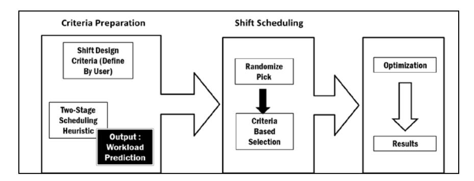
Figure 1 Proposed architecture.
A set of parameters defined by the user is used to generate all possible shifts. The shifts are assigned accordingly to form schedules. The list of schedules is then processed using two separate methods to identify efficient schedules in order to increase the chances of obtaining the 'best' schedule candidates within a short time frame. All the selected schedules are then optimized as best as possible to cover all jobs with minimum manpower and the least wastage. Figure 2 illustrates the shift scheduling process.
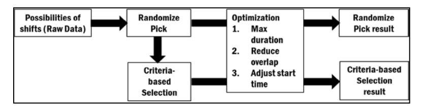
Figure 2 Shift scheduling process.
3.1 Random Pick
This process applies a simple random pick method with the goal of selecting good schedules from all possible shifts available. Recursive randomization is also implemented to reduce the number of potential candidate schedules with the intention of keeping good schedules among good candidate schedules that have been identified. The implementation of the random pick function is documented in Figure 3.
Random pick function
for i = 0, .....ShiftMax do
 MorningShift.Add(Random(MorningCandidate));
 DayShift.Add(Random(DayCandidate));
 AfternoonShift.Add(Random(AfternoonCandidate));
 NightShift.Add(Random(NightCandidate));
end for
Schedule = CreateSchedule(MorningShift, DayShift, AfternoonShift, NightShift);
CalculatePenalty(Schedule);
Optimize(Schedule);
Present(Schedule);
Figure 3 Random pick function.
The algorithm generates all possible shifts and then pairs them randomly to form a schedule. The possible candidates of schedules will be pre-processed, optimized and presented prior to the process of selecting the best schedule.
3.2 Criteria-based Selection
Criteria-based selection is aimed at picking schedules that fulfill certain required criteria, such as minimum manpower, minimum duration or the earliest/latest starting time of a shift as in Eqs. (1) to (3).
\[\alpha^{\min/\max} = \min/\max(\{f(x): x = 1, ...., n\}), \alpha = resource\] (1)
\[\beta^{\min/\max} = \min/\max(\{f(y): y = 1, \dots, n\}), \beta = duration\] (2)
\[\gamma^{\text{earliest/latest}} = \min/\max(\{f(z): z = 1, \dots, n\}), \gamma = \text{starttime}\] (3)
48 combinations of criteria are identified and then used to determine the 'good' schedule candidates for the next selection process. The list of criteria combinations can be found in Eqs. (4) to (9):
\[\alpha^{\min/\max} > \beta^{\min/\max} > \gamma^{earliest/latest}\] (4)
\[\beta^{mix/max} > \gamma^{earliest/latest} > \alpha^{min/max}\] (5)
\[\beta^{mix/max} > \alpha^{min/max} > \gamma^{earliest/latest}\] (6)
\[\gamma^{\text{earliest/latest}} > \beta^{\text{mix/max}} > \alpha^{\text{min/max}}\] (7)
\[\gamma^{earliest/latest} > \alpha^{\min/\max} > \beta^{\min/\max}\] (8)
\[\alpha^{\min/\max} > \gamma^{earliest/latest} > \beta^{\min/\max}\] (9)
From these selections of criteria, the number candidates of 'good' schedules picked is 48. The intentions of applying the criteria-based selection are to evaluate and discover the criteria that most likely influence the best solution. The implementation of the algorithm based on the methods explained is as shown in Figure 4.
Criteria-based selection function (minimum resource αmin)
minResources = -1;
for m = 0, .....resources.Count
 if uncover[m] == minUncovered then
 if minResources == -1 then
 minResources = resources[m];
 index = m;
 else
 if minResources > resources[m] then
 minResources = resources[m];
 index = m;
 end if
 end if
 end if
 end for
Figure 4 Criteria-based selection function.
The implementation of the algorithm shown in Figure 4 was extended to cover the rest of the possibilities in order to produce the best solutions for each criterion determined before.
3.3 Optimization
Good schedule candidates picked or selected from both the randomized and criteria-based selections are optimized to improve the quality of the schedules. The objectives of the optimization are aimed at reducing the use of resource/manpower, avoiding overlaps of shift periods and uncovered jobs. The algorithm for optimization is as shown in Figure 5.
Optimization function
for i = 0, .....ScheduleMax do
 for j = 0, .....ShiftMax do
 e1 = GetStartTime(Schedule[i][j]);
 e2 = GetFirstJobStartTime(jobs);
 if e1 >= e2 then
         newStartTime = e2
 else
 newStartTime = e1
 end if
 Schedule[i][j] = VerifyTruncateStartTime(newStartTime);
 d1 = Schedule[i][j].Duration;
 d2 = MaxShiftLength(Schedule[i][j+1]);
 if d1 >= d2 then
 newDuration = d1
 else
 newDuration = d2
 end if
 Schedule[i][j] = VerifyTruncateEndTime(newDuration);
 if j == ShiftMax then
 Schedule[i][j] = VerifyTruncateEndTime(maxDuration);
 end if
 end for
end for
Figure 5 Optimization function.
Initially, the algorithm tries to optimize the duration within the permitted time window to cover more jobs while avoiding overlap of shifts. Next, it tries to adjust the starting time to reduce overlap of shifts while respecting the time window restriction. Lastly, it tries to cover all jobs by pushing the starting times of previous shifts even though the benefit is for the subsequent shifts. All the optimizations avoid overlapping with other shifts and stay within the range of parameters defined by the user. The optimization steps are repeated until there is no more improvement. Finally, the good schedule candidate is considered optimized and ready to be placed in the evaluation pool.
4 Simulation
Real problem data collected from an airline company based in Malaysia (KLIA) were investigated. Table 1 shows an example of a shift schedule.
| Day 1 | Day 2 | Day 3 | Day 4 |
|---|---|---|---|
| 0700-1700 | 0700-1700 | 0700-1600 | 0700-1600 |
| 1500-2400 | 1500-2400 | 1600-2400 | 1600-2400 |
| 2200-0700 | 2200-0700 | 2200-0700 | 2200-0700 |
Table 1 Manually assigned shifts.
To conduct a sensitivity analysis of the proposed algorithm, real problem datasets were used to generate shift scheduling with different starting time ranges. Aside from that, job demand data were also collected, as shown in Table 2. Job demand data are vital information needed by the proposed algorithm to ensure that the shifts created take into consideration all jobs available and wastage is reduced.
| Job ID | Release Time | Deadline | Processing Time | Number of Tasks |
|---|---|---|---|---|
| 1 | 0 | 4 | 3 | 1 |
| 2 | 0 | 4 | 3 | 1 |
| 3 | 90 | 98 | 5 | 1 |
| 4 | 90 | 98 | 5 | 1 |
| 5 | 96 | 100 | 1 | 1 |
Table 2 Job demand data.
4.1 Criteria Preparation
The initial step toward the solution is to generate an optimum workload prediction using TSH. Shifts cannot be implemented based on workload prediction because then it will generate different manpower allocations for different periods. However, workload prediction can be used as a guide to generate an optimum schedule. User input of shift design criteria is used to list out all possibilities of schedules with all combinations of starting times and durations. The list of raw schedules along with the result of workload prediction form the input for the shift scheduling algorithm to schedule shifts.
4.2 Shift Design Criteria
In shift scheduling, a shift is known as the time interval defined by beginning time, ending time and duration. A one-day shift time comprises four shifts, i.e. morning, day, afternoon and night. For each of the shift times, the user is able to choose the earliest starting time, latest starting time, minimum duration and maximum duration, as illustrated in Figure 6.
Figure 6 Defining a day shift time.
Two different ranges for the starting time, namely between 2 hours and 4 hours, were used to analyze the performance of the method. The starting time range refers to the difference between the earliest starting time and the latest starting time. For the 2-hour range of the morning shift, the earliest starting time (EST) was 0500 and the latest starting time (LST) was 0700. The logic of having a 2 hour range is to simulate a loosely restricted starting time range so that the shift is more adaptable to employees. The 4-hour range was formed to test whether relaxation of the starting time range would yield a schedule that is more cost effective and provide less wastage, which should be the case in theory.
| Shift Starting time | 2 hours' range (EST – LST) | 4 hours' range (EST – LST) |
|---|---|---|
| Morning | 0500 – 0700 | 0300 – 0700 |
| Day | 1000 – 1200 | 0800 – 1200 |
| Afternoon | 1600 – 1800 | 1400 – 1800 |
| Night | 2100 – 2300 | 1900 - 2300 |
Table 3 Shift starting time range used for testing.
5 Computational Results
The results presented in this section were obtained based on the data from a real problem found in an international airport in Malaysia. The real problem datasets contained 1023 jobs; each job had the following attributes: job number, release time, deadline and processing time. The data sets comprised a collection of the real number of jobs for the first four days of the week. Due to unforeseen circumstances, the datasets were incomplete as the records for the last three
days of the week were missing. Nevertheless, the algorithm managed to simulate and produce the desired result even with only four days of datasets.
In this case study, a prototype was developed using C# from scratch. All experiments were carried out on a Toshiba laptop with Intel® CORETM i5 2.4GHz and 8GB memory. In addition to testing on the 4-day datasets, which comprised 1023 jobs, testing was also done with 1-day datasets, which consisted of 234 jobs. All experimental tests generated the result in less than thirty seconds, as shown in Table 4.
Table 4 Computational time with different dataset sizes.
| Schedule | Average (s) |
|---|---|
| 1 day | 4.72 |
| 4 days | 29.27 |
5.1 Performance Analysis
The schedules generated by the proposed algorithm are as shown in Table 5.
Table 5 Shift schedules from the proposed algorithm.
Parameters starting time range = 2 & 4 hours • manpower = 310 • overlapped duration = 7:45 hours • manpower = 316 • overlapped duration = 8 hours
| Random pick | Criteria-based Selection | |||||
|---|---|---|---|---|---|---|
| 0700-1300 0700-1300 0645-1245 0700-1300 0700-1300 0700-1300 0700-1300 0700-1300 | ||||||
| 1200-1800 1200-1800 1200-1800 1200-1800 1200-1800 1200-1800 1200-1800 1200-1800 | ||||||
| 1800-2400 1800-2400 1800-2400 1800-2400 1800-2400 1800-2400 1800-2400 1800-2400 | ||||||
| 2300-0700 2300-0645 2300-0700 2300-0900 2300-0700 2300-0700 2300-0700 2300-0900 | ||||||
Our test revealed that the starting time range in this scenario did not impact the schedule selected. The random pick algorithm performed slightly better, with a reduction in the number of manpower/resources required and overlapping shift time. The criteria-based selection did not perform as well as the randomized pick algorithm, as the former algorithm needed to adhere to a stricter criteria limit. The highlighted cells indicate the difference between two scheduled shifts from different solutions. The CBS algorithm consistently picked the same starting time while the RP algorithm proved true to its nature by picking without restriction, which led to the outlier in shift starting time. Results obtained from the proposed algorithms with TSH and manual schedule shifts are shown in Figure 7.
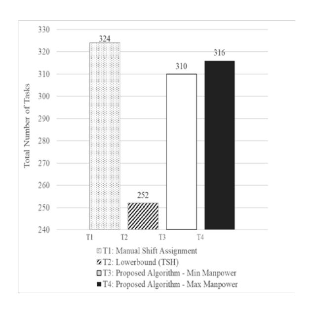
Figure 7 Comparison between manpower requirements produced by manual, lower bound, and proposed method.
In summary, the manpower required by the proposed shift scheduling algorithms was lower than that required by the manually assigned shifts, namely a reduction between 2.47% and 4.32%. If 2.47% of reduction is translated into current monetary gain, it would be equivalent to USD 12.5K of savings per annum.
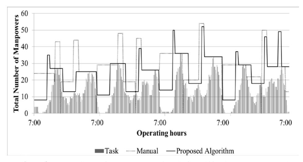
Figure 8 Comparison of manpower assigned for shifts between proposed algorithm vs manual assignment.
The chart in Figure 8 shows that the proposed algorithm projected a starting time pattern that was quite consistent throughout the week, which indicates that the resources were being utilized efficiently according to the workload distribution. The peak exhibited in the chart indicates an overlap of shifts that implies wastage of resources. The chart shows that the proposed algorithm produced fewer peaks compared to the manual shift scheduling.
5.2 Sensitivity Analysis
To examine the impact of the shift starting time and duration, the same test on was used on the same datasets to run the algorithm while disregarding the constraints individually. The sensitivity results are summarized in Figure 9 and Figure 10.
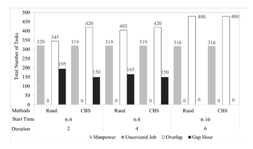
Figure 9 Relation between resource values vs different range of shift starting time and duration.
The same datasets were run using the same algorithm but with a different range of starting time and shift duration. The wider the range and the longer the duration, the lower the number of manpower/resources required to complete all the jobs, as shown in Figure 9. The manpower reduced from 320 to 316 as the range for starting time and shift duration widened. This is expected, as a relaxation of constraints provides the possibility of designing better shifts. The wider range of the constraints, especially shift duration, also causes overlapping of shifts. This is due to the starting time, which is a restricted constraint defined at the input stage. The difference between the starting time was also reduced when the constraints were relaxed, namely the value dropped from 195 to 150 and eventually to zero, which indicates that all the shifts have the same starting time. Besides showing manpower reduction when compared to manual
scheduling, both algorithms are also able to reduce the overlapping between shifts if the appropriate duration range was defined. The CBS algorithm showed that it has the advantage of assigning the shift starting time range in a consistent manner, which is a trait desired by employees.
Next the same test was repeated, but with a fixed shift range duration of 5, 6 and 8 hours. A difference was observed in the starting time range, where three ranges of starting time were tested. The trend indicates that the range of the starting time did not impact either the uncovered jobs or the overlap of shift values. Instead, the duration of the shift played an important role here. As shown in Figure 9, the longer the shift duration, the higher the value of overlapping of shifts. However, it was the opposite for uncovered jobs, where the trend shows that the shorter the shift duration, the higher the value of uncovered jobs, which makes perfect sense. Shorter shifts could be designed but this cannot handle the available jobs, as shown in Figure 10.
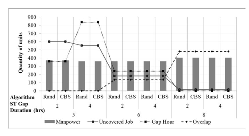
Figure 10 Relation between uncovered jobs and overlapping shifts vs different ranges of shift starting time and duration.
Figure 11 shows that shift duration is essential in determining the required number of manpower/resources. A long sift duration causes shift overlap, as shown in this test, where 8 hours was defined as shift duration with four shifts per day. Overly short shift durations have the same impact, but in this instance, the value is not as bad as when the shift duration is long. The optimum number of manpower was achieved when the shift duration was six hours. This is logical as four shifts with 6-hour shifts would cover the whole day's jobs.
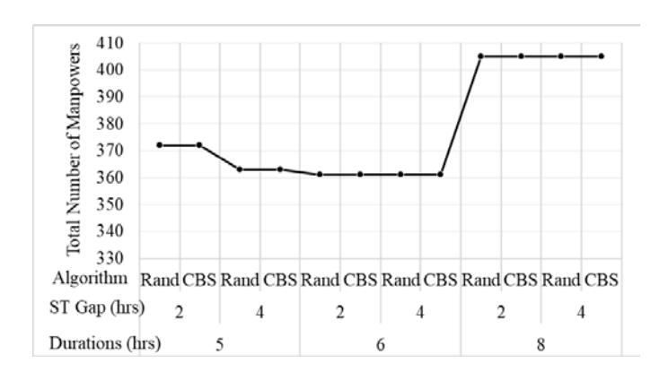
Figure 11 Relation between manpower/resource vs different ranges of shift starting time and duration.
6 Discussion
Real-world scenarios provided by an industrial partner, as mentioned in the above section, were used. The dataset consisted of 4-day instances for a total of 1023 job instances. The simulated dataset comprising of the original dataset with extended random generated data was also tested. Multiple experiments were conducted to evaluate the effectiveness of the different components of the proposed algorithm and its performance. In this section, a discussion is presented of the results generated by the solution applied using our approach algorithm as compared to a well-known genetic algorithm (GA). The results of the comparisons are shown in Figure 9 and Tables 6 to 8.
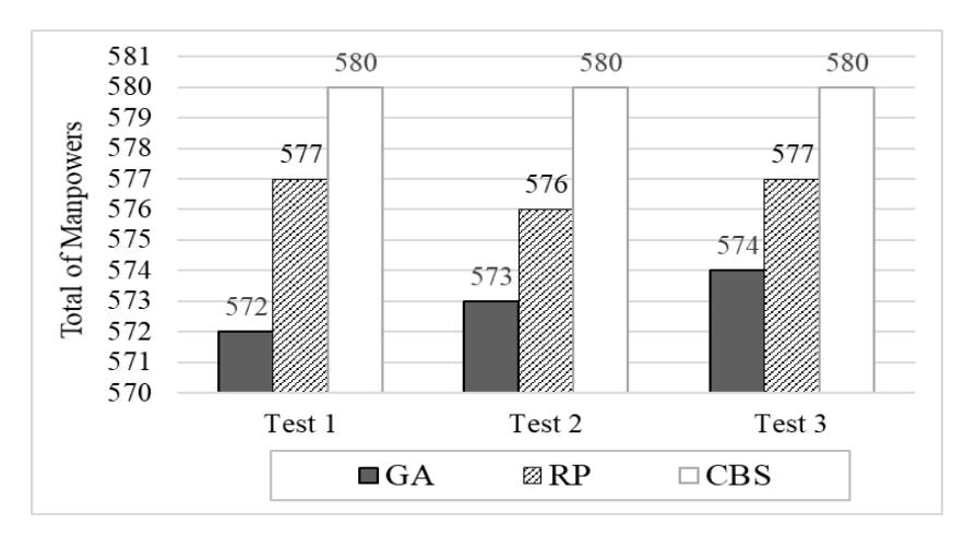
Figure 12 Comparison of manpower utilization, the less the better.
The results in Figure 9 reveal that good-quality solutions could be obtained with all three methods. Additionally, the results also show that GA produced slightly better results, namely up to 0.17% lesser manpower to complete the same number of jobs. But the comparison of solution time of the algorithms indicates that the heuristic algorithm yielded results faster and required less time to achieve high-quality, distributed and uniform solutions when compared to GA.
Table 6 Uncovered jobs values for GA, RP and CBS.
| Algorithms | Test 1 | Test 2 | Test 3 |
|---|---|---|---|
| GA | 15853 | 4608 | 7474 |
| RP | 0 | 0 | 0 |
| CBS | 0 | 0 | 0 |
Table 7 Overlapping shift durations for GA, RP, and CBS.
| Algorithms | Test 1 | Test 2 | Test 3 |
|---|---|---|---|
| GA | 1499 | 553 | 1169 |
| RP | 124 | 125 | 122 |
| CBS | 116 | 116 | 116 |
Table 8 Gap hour duration values for GA, RP and CBS.
| Algorithms | Test 1 | Test 2 | Test 3 |
|---|---|---|---|
| GA | 10245 | 5970 | 7365 |
| RP | 22 | 18 | 1 |
| CBS | 2 | 2 | 2 |
Aside from manpower, the GA method also failed to produce good results for other objectives, such as covering all jobs available, as shown in Table 6. GA also generated the schedule with the highest number of unutilized resources, such as idling manpower during working hours, and the results obtained were consistent, as clearly indicated in Table 7. On the other hand, the proposed heuristic algorithm generated shift schedules that managed to maintain a 'respectable' amount of manpower with minimum uncovered jobs and overlapping shifts. Lastly, the proposed algorithm demonstrated the ability to assign consistent shift starting times, as highlighted in Table 8, which would ensure a fair schedule as well as higher adaptability of the employees to the schedule. Hence, the results showed that the proposed algorithm can obtain high-quality results with less computational resources.
7 Conclusion
In this paper, an algorithm to design shift schedules was presented and successfully applied to real airline data. The algorithm employed two methods: random pick and criteria-based selection to design the shift schedule. The shift schedule designed by both techniques was optimized using requirements provided to reduce the use of resource/manpower, reduce overlapping of shift periods and uncovered jobs. The proposed algorithm demonstrated the ability to generate very high-quality solutions within short span of time. Specifically, the algorithm managed to reduce up to 4.32% of resource utilization and up to 30% of shift duration overlaps. Furthermore, the proposed algorithm exhibited the capability of solving large problem instances in less than a minute. The results suggest that further improvement can be achieved, especially in reduction of resources. Future studies may consider exploring and taking advantage of the shift change period to optimize manpower utilization between two shifts to reduce it. As machine learning has gained popularity in solving various types of problems, this area of study can also be applied to shift scheduling problems.
Acknowledgments
This work was supported and funded by the Ministry of Higher Education, Malaysia under grant number of FRGS/ICT07(03)/1202/2014(03).