
1 Introduction
Optical communications systems that use advanced modulation schemes such as M-ary Quadrature Amplitude Modulation (M-QAM) have increased in optical communication networks over nearly a decade [1]. For this reason, researchers have attempted to improve the performance of these systems by applying several different techniques to achieve a high quality of service [2,3].
Recently, artificial intelligence (AI) techniques have been applied to optimize the performance of optical communication systems [4-6]. For example, artificial neural networks (ANNs) [7], convolutional neural networks (CNNs) [8], deep neural networks (DNNs), and principal component analysis (PCA) [9]. These neural network techniques have been proposed to enhance the optical performance monitoring (OPM), including optical signal to noise ratio (OSNR), chromatic dispersion (CD), and polarization mode dispersion (PMD) [10]; and mitigation of nonlinear distortion [2,11]. Modulation formats (MFs) enhanced for a coherent detection receiver using a deep neural network (DNN) based on an asynchronous amplitude histogram was obtained after constant modulus algorithm (CMA) equalization to identify three modulation schemes with good accuracy in [9]. Also, a deep learning algorithm based on an intelligent eyediagram analyzer to implement modulation format identification (MFI) has been proposed in [12]. Furthermore, MFs were identified for different QAM modulation forms with indirect detection receiver using an artificial neural network (ANN) for elastic optical networks [13].
In this paper, seven different training algorithms for feed-forward artificial neural networks (ANNs) are proposed to optimize the performance of coherent optical communication systems with four modulation schemes at high data rates, including 240Gbps dual-polarization (DP) 16-QAM, 240Gbps DP-64-QAM, 240Gbps DP-128-QAM, and 240Gbps DP-256-QAM as signal codes. The proposed approach uses a multi-layered neural network with back-propagation (BP) as the training algorithm.
2 Optimization Methods
In a feed-forward ANN model, the network is constructed using layers as represented in Figure 1 [14]. The input vector passes through the network layer by layer until the output layer is reached. There is only one input node in the first layer. The second layer is a hidden layer takes place in the second layer, it contains nonlinear units that are connected directly to the input node. According to Eq. (1) there are 20 nodes in the hidden layer [15]:
\[Nh \ge (2Ni + 1) \tag{1}\] where Nh represents the number of nodes in the hidden layer and Ni is the number of nodes in the input layer. The weights between the input layer and the hidden layer are \(w_{ij}\) (i = 1, 2, ..., Nh); (j = 1, 2, ..., Nh), and the thresholds are \(\theta j\). Similarly, the weights between the hidden layer and the output layer are \(w_{jk}\) (k = 1, 2, ..., no), and the thresholds are \(\theta_k\). The outputs of each layer are given by [16]:
\[x_j' = f_1 \left( \sum_{i=1}^{Ni} w_{ij} x_i - \theta_j \right) \tag{2}\]
\[y_k = f_2 \left( \sum_{j=1}^{Nh} w_{jk} x_j - \theta_k \right) \tag{3}\]
The activation function of the individual hidden units in the NN is hard-limit [17]:
\[F_1(z)=1 \text{ if } z \ge 0,\] and the activation functions of the output layer is log-sigmoid [17]:
\[F_2(z) = 1 / (1 + \exp(-n))\]
The last layer is the output layer, which consists of one node. For updating the weights of the NN, several training methods were used, i.e.:
- 1. OSS: One Step Secant [18]
- 2. CGF: Conjugate Gradient with Fletcher-Powell Conjugate Gradient [19]
- 3. BFG: BFGS (Broyden Fletcher Goldfarb Shanno) Quasi-Newton [20]
- 4. RP: Resilient Backpropagation [21]
- 5. LM: Levenberg-Marquardt [19]
- 6. SCG: Scaled Conjugate Gradient [22]
- 7. CGP: Conjugate Gradient Backpropagation with Polak-Ribiére [19].
Figure 1 The structure of an artificial neural network.
3 Simulation Setup and Results
The simulation setup used is shown in Figure 2. First, a huge bit sequence (240Gbps) is generated by PRBS (pseudo-random bit sequence), which then is converted from serial to parallel sequences to produce dual-polarization multilevel quadrature amplitude modulation electrical signals like DP-16-QAM, DP-64-QAM, DP-128-QAM, and DP-256-QAM. Second, an optical carrier is modulated with M-QAM signals at 1550 nm center frequency, and then the dualpolarization optical signals are combined by using Polarization Combiner (PC).
Then, the amplified optical signal is transmitted over a recirculating loop fiber consisting of an 80-km span of standard single-mode fiber (SSMF) and an erbium-doped fiber amplifier (EDFA). After that, the optical signal output from the fiber loop is filtered by a (0.4 nm and 50 GHz) bandwidth optical bandpass filter (OBPF) to cancel redundant noise present in the signal. At the receiver side, the received optical signal is divided into two polarized signals by a polarization splitter, and then is detected coherently by a coherent optical receiver.
The values of the simulation parameters used in the system are shown in Table 1. The detected signals were sampled to collect 4194304 samples for DP-16QAM, DP-64QAM, DP-128QAM, and 8388608 samples for DP-256QAM in one sequence and then processed offline by utilizing the seven different training algorithms for the feed-forward artificial neural networks (ANNs). The commercial software Optisystem was used to simulate this optical system, and MATLAB for offline processing.
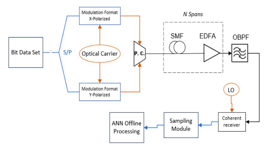
Figure 2 The simulation setup of an DP-M-QAM optical communication system.
| Parameters | Values | Parameters | Values |
|---|---|---|---|
| Data rate | 240 Gbps | Fiber attenuation | 0.2 dB/km |
| Optical Power | -5 ~ +5 dBm | Dispersion coefficient | 16.75 ps/nm.km |
| Linewidth of optical carrier | 100 kHz | Nonlinear index of refraction | 26e-021 m2/W |
| Linewidth of local oscillator | 100 kHz | One span fiber length | 80 km |
| EDFA gain | 20 dB | EDFA noise figure | 4 dB |
Table 1 Simulation system parameters values.
The identification accuracy results of four modulation formats, DP-16QAM, DP-64QAM, DP-128QAM, and DP-256QAM, are summarized in Table 2. According to Table 2, the obtained results showed identification by the four proposed modulation schemes at 100% accuracy when using the BFG and OSS neural network training algorithms. Figure 3 shows the accuracy of identification against OSNR. The OSNR alternates between 10 and 35 dB. High identification accuracy was observed for the DP-16QAM, DP-64QAM, and DP-128QAM at 13 dB OSNR, while high identification accuracy for the DP-265QAM was observed at about 22 dB OSNR.
Table 2 Identification accuracies of the four used modulation schemes using the proposed artificial neural network training algorithms.
| Accuracy of Identification | ||||||
|---|---|---|---|---|---|---|
| NN Training algorithms | 16-QAM at OSNR=19dB | 64-QAM at OSNR=25dB | 128-QAM at OSNR=26dB | 256-QAM at OSNR=30dB | ||
| BFG | 100% | 100% | 100% | 100% | ||
| OSS | 100% | 100% | 99.99% | 100% | ||
| LM | 99.90% | 97.10% | 99.28% | 96.80% | ||
| SCG | 88.90% | 62.30% | 65.90% | 67.65% | ||
| CGF | 100% | 100% | 99.95% | 99.80% | ||
| CGP | 100% | 100% | 99.99% | 99.90% | ||
| RP | 77.50% | 75.70% | 75.40% | 56.75% | ||
This section illustrates the performance of the seven training functions and the original signals of the four modulation schemes. The OSS algorithm achieved the best convergence of OSS algorithm. This NN algorithm had a noticeable advantage, because it requires very accurate training. The smallest lower mean square errors among the other algorithms tested could be obtained using the BFG training method. The LM algorithm had larger storage requirements than the other algorithms tested. The advantage of LM decreased when the number of weights in the network was increased.
The performance of CGF was similar to the performance of BFG. It has an advantage over the LM method, because it does not require high storage. On the other hand, a drawback is that the computation required increases by a constant ratio with the size of the network, because the equivalent of an inverse matrix must be computed at each iteration. The CGP algorithm performance was faster than CGF and its accuracy was almost the same as that of the OSS algorithm. The performance of conjugate gradient algorithm SCG was good over a wide set of problems. By comparing the performance of SCG and LM, unlike LM, the performance of SCG did not degrade quickly when the error was reduced. The conjugate gradient methods have comparatively moderate storage requirements.
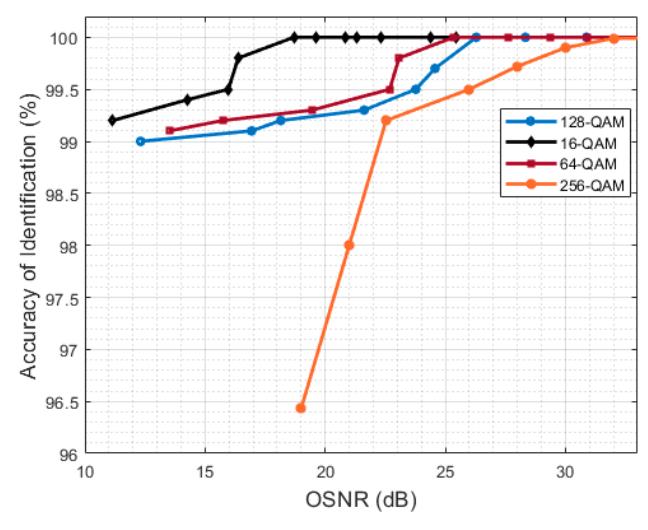
Figure 3 Identification accuracy for four modulation scheme curves versus OSNR using the BFG NN training algorithm.
Compared with the other algorithms, they were usually the slowest. Meanwhile, the performance of the RP method degraded as the error target was reduced. For this method, the storage requirements are comparatively low compared with the other methods. The performance of the RP method was similar to that of the LM algorithm, with almost the same speed of convergence, and its accuracy was almost the same as that of the SCG algorithm. Table 3 contains the performance of the seven NN training methods. The results were taken for four types of modulation schemes, DP-16QAM, DP-64QAM, DP-128QAM, and DP-256QAM. The results show the values of mean square error (MSE) for each algorithm. The error is the difference between the calculated output and the goal. The convergence speeds of the BP training algorithms were between (3-180) epoch, i.e. the best convergence speed among the (CGF, BFG and OSS) methods.
| Table 3 | MSE performance of the seven NN algorithms. |
|---|
| NN Training Algorithms | 16-QAM | 64-QAM | 128-QAM | 256-QAM |
|---|---|---|---|---|
| BFG | 10-30 | 10-23 | 10-14 | 10-12 |
| CGF | 10-17 | 10-15 | 10-10 | 10-10 |
| CGP | 10-23 | 10-13 | 10-12 | 10-12 |
| LM | 10-10 | 10-7 | 10-9 | 10-9 |
| OSS | 10-22 | 10-21 | 10-13 | 10-12 |
| RP | 10-8 | 10-8 | 10-7 | 10-7 |
| SCG | 10-7 | 10-8 | 10-7 | 10-8 |
4 Conclusions
In this work, seven training algorithms for feed-forward artificial neural networks (ANNs) have been proposed to identify the performance of four modulation schemes, DP-16QAM, DP-64QAM, DP-128QAM, and DP-256QAM, in an optical system. The neural training algorithms (CGF, BFG, CGP, and OSS) gave better symmetry than the other neural training methods proposed in this work. The proposed approach is to take one node for samples serially rather than several nodes with one sample in parallel. The results from the first approach gave higher accuracy for symmetry.