
1 Introduction
Wireless sensor networks (WSN) are self-organizing, distributed, scalable networks consisting of many autonomous sensors (sensor nodes) that are united through a radio channel. The nodes are autonomous in terms of power supply, maintenance staff is not required to keep up the network, and the network can be rebuilt over time [1-5]. To date, some of the nodes of the total number of internetconnected things are WSN nodes. This is due to the fact that the latter are one of the directions in the development of the Internet of Things, providing ample opportunities for integration into various processes [2]. There are several key
problems in the self-organization and routing of data in WSN: in selforganization, some nodes may not be involved and may be outside the network [3]; many routing protocols are not able to adapt to changes in the location of the base station (BS) [4]; in 'flat' protocols the energy of all intermediate nodes is consumed when transferring data from node A to node B, which negatively affects the lifetime of the entire network [5]; in many hierarchical protocols, all or part of the nodes included in a cluster often cannot transmit data among themselves, since clustering does not use the radio visibility of the nodes but their coordinates obtained via GPS/GLONASS [6]. For hierarchical protocols to build a hierarchy, one of the main tasks is the clustering of nodes, since scalability and network performance depend on it.
WSN clustering refers to the separation of network nodes into separate groups (clusters), each of which is assigned a main cluster node (MCN), routing data between cluster nodes, and transmitting aggregated data to the BS. The developed routing protocol can use a neural network and matrix clustering. The protocol allows optimizing data transmission in the network, increasing its lifetime and survivability. The hierarchical orientation of the protocol provides high scalability of the network (up to 10,000 nodes or more) and allows the use of a mobile base station [6]. Using the mechanism of an artificial neural network allows to effectively cluster the nodes of the wireless sensor network, taking into account many different parameters: the level of radio visibility, the level of residual energy, the priority of nodes, etc.
Table 1 Routing protocols of wireless sensor networks (WSN).
| Protocol Category | Protocols | |||
|---|---|---|---|---|
| Based on the location of the nodes | MECN, SMECN, GAF, GEAR, Span, TBF, BVGF, GeRaF | |||
| Directional on aggregated data | SPIN, Directed Diffusion, Rumor Routing, COUGAR, ACQUIRE, EAD, Information-Directed Routing, Gradient-Based Routing, Energy-aware Routing, Information-Directed Routing, Quorum Based Information Dissemination, Home Agent Based Information Dissemination | |||
| Hierarchical | LEACH, PEGASIS, HEED, TEEN, APTEEN | |||
| Based on mobility | SEAD, TTDD, Joint Mobility and Routing, Data MULES, Dynamic Proxy Tree-Base Data Dissemination | |||
| Multi-oriented | Sensor-Disjoint Multipath, Braided Multipath, N-to-1 Multipath Discovery | |||
| Based on heterogeneity | IDSQ, CADR, CHR | |||
| Based on quality of service (QoS) | SAR, SPEED, Energy-aware routing | |||
The routing protocols for WSN are responsible for supporting the routes in the network and must guarantee reliable communications even in severely adverse conditions. Many protocols for routing, power management and data distribution have been specially developed for WSN, where energy saving is a significant problem, which the current protocol aims to solve [7]. Others were designed for general use in wireless networks but also found application in WSN. A classification of WSN protocols [8] is presented in Table 1 [9].
2 Problem Statement
In hierarchical protocols (clustering-based protocols), a network is divided into clusters (groups of nodes). This allows more efficient use of the energy resources of the network, thereby prolonging its life cycle. In hierarchical protocols, a separate place is occupied by the concept of connectivity. Connectivity is divided into two categories: intra-cluster and inter-cluster connectivity. Intra-cluster connectivity ensures data transfer between nodes within a cluster, while intercluster ensures connectivity between other clusters as well as the BS [10,11]. One of the main problems in the development of routing protocols for WSN is their energy efficiency due to the limited energy resources of the sensor nodes. The protocol should keep the network up and running as long as possible, thereby prolonging the network's life cycle.
Routing protocols play a significant role in the functioning of WSN. Thanks to them, self-organization of nodes and packet delivery by optimal routes are carried out in accordance with the algorithms used in the corresponding protocol. By choosing an effective routing protocol it is possible to optimize the use of network resources, such as power consumption, processor time, memory, etc. Therefore, the use of an effective routing protocol allows to maximize the network's life cycle.
An artificial neural network (ANN) is a model of a biological nervous system and represents a network of interconnected nodes with activation functions, called neurons. All types of neural networks are obtained by varying the activation functions and the weights of the connections between the neurons [12].
Tasks that ANNs can solve in wireless sensor networks:
Clustering. One of the methods for extending the life cycle of a network as well as methods for transmitting packets is the clustering method, which is used in many routing protocols for WSN. Clustering can be performed nonlinearly, using an ANN that can optimally divide sensor nodes into clusters in accordance with specified criteria (radio visibility level, geographical coordinates, residual energy level, etc.).
Routing. Routing can be done through artificial intelligence. One use example is multi-path routing, where the route that is most optimal in terms of the data delivery speed is estimated using an ANN and a number of criteria.
Prediction of the life cycle of a sensor network. The life cycle of a network can be estimated by a number of characteristics of its nodes and by the type and frequency of data transmission. An ANN can perform an approximation of the operation of the entire network in order to predict what characteristics both the entire network and its individual components will have over a certain period of time of its functioning [13].
Analysis and traffic management. ANNs are able to analyze traffic and to cluster it, thereby determining what type of data is transmitted. Based on this, the neural network can make decisions about narrowing the channel or providing the necessary bandwidth.
Network error detection. This sets a set of indicators of key parameters, where the neural network checks their values with ideal values over time, on the basis of which the ANN is trained. Based on comparison, the neural network decides whether the network works efficiently to accomplish a task. The tasks of clustering, routing and forecasting the life cycle of the sensor network were used in the present work.
An ANN initially goes through a training phase where it learns to recognize patterns in data, whether visually, aurally, or textually. During this supervised phase, the network compares its actual output produced with what it was meant to produce (the desired output). The difference between both outcomes is adjusted using back propagation. This means that the network works backward, going from the output unit to the input units to adjust the weight of its connections between the units until the difference between the actual and the desired outcome has the lowest possible error [14].
3 Problem Decision
A wireless sensor network can be considered an ANN if we assume that each of the ANN inputs receives values using sensory nodes that convert the values of the physical world into electrical signals, which are digitized and then are transmitted to program-modeled neurons as vector input quantities (see Figure 1).
3.1 Neural Wireless Sensor Network
Such a neural network will make decisions based on the input values of the WSN, which serves as a mobile, independent, self-organizing body for connecting the neural network with the real world [15].
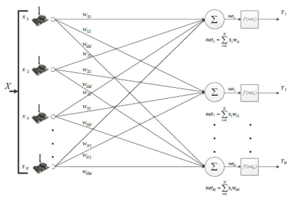
Figure 1 Neural wireless sensor network.
Designations used in Figure 1: X is the input layer of neurons containing the components of the input vector; N is the number of input neurons (network inputs), \(x_1, x_2, x_3, ..., x_N\)-number of clusters; \(w_{11}, ..., w_{NM}\)- neuron weight; \(\Sigma\)-Kohonen layer, which consists of linear weighted adders and implements the main mathematical apparatus of the ANN; \(f(net_1), ..., f(net_M)\) is the output function of the neural network formed after the function of summation and other mathematical transformations; \(Y_1, Y_2, ..., Y_M\) is the output layer, containing the components of the output vector, whose neurons transmit output signals. An interpreter is placed at the output of the network, which determines to which class the input vector belongs based on the magnitude of the signal.
To solve the problem of routing in a wireless sensor network based on a neural mechanism, the Kohonen ANN was selected. This choice was due to the lack of deficiencies that are inherent to neural networks that are similar in methodology to teaching without a teacher. The existing shortcomings of the Kohonen ANN were eliminated through the use of the constructive method as training method.
3.2 Substantiation
A radio visibility matrix is proposed, which is a mathematical description of the connectivity of network nodes and the radio visibility of each node with respect to all other network nodes. This mathematical representation allows to describe all the nodes of the network and prepare data for the corresponding form to be input into the ANN. Based on the Kohonen ANN trained by the constructive method [13,14], a method for neural network clustering of WSN was developed [15]. A matrix method for clustering WSN was also developed. To effectively use the developed method of neural network clustering, a hierarchical data routing protocol for WSN was developed.
Each WSN node has its own set of neighbors: = {} = 1, … . , , … , , ∈ where is the power of multiple neighbor nodes . The set may be empty if node is isolated ( ∈ ∅). To each neighboring node from the set Z corresponds to the power level of the received signal (RSS, received signal strength) [16] relative to the node that owns the set of neighbor nodes . Thus, each node has its own power vector ⃗, where each power level corresponds to a certain neighboring node from the set (Eq. (1)):
\[\vec{p}_i \in Z_i = \{p\} \in \{z\} = p_1 \in z_1, \dots, p_j \in z_j, \dots, p_L \in z_L\] (1)
Consequently in the following Eq. (2),
\[\forall q_i \exists Z_i \in q_i : (p_1 \in z_1, \dots, p_j \in z_j, \dots, p_L \in z_L) \in q_i\] (2)
3.3 Formation of a Mathematical Model
We use the mathematical description of the WSN nodes 1, … , in the form of the radio visibility matrix P. For the radio visibility matrix P, we normalize all values using the following Eq. (3):
\[p_{NORM} = \frac{p}{p_{MAX}},\tag{3}\] where is the maximum power level of the signal node i with respect to node j, = 100.
For the operation of the neural network and matrix methods of clustering it is necessary to first present the data in the form of a radio visibility matrix, which is a mathematical description of the WSN nodes and reflects the level of radio visibility between all nodes in a percentage ratio. Radio visibility matrix P (energy visibility matrix, matrix radio communications, power matrix) is a square
matrix of order N that describes the connectivity between the nodes of the wireless network, where each node \(q_i\) is in matching multiple RSS (received signal strength) signal strengths \(\{p\}\) it neighbors node \(\{z\}\).
Each row of matrix P is an input vector for a neural network and carries information about each of the network nodes and about its visibility relative to the other network nodes. Using this matrix, we can describe graph \(G = \{Q, P\}\), where Q are many sensor nodes, P are many signal power levels [17].
We get the normalized matrix of radio visibility in Eq. (4) as follows:
\[P_{NORM} = \begin{pmatrix} 1 & \frac{p_{12}}{p_{MAX}} & \dots & \frac{p_{1j}}{p_{MAX}} & \dots & \frac{p_{1n}}{p_{MAX}} \\ \frac{p_{21}}{p_{MAX}} & 1 & \dots & \dots & \frac{p_{2j}}{p_{MAX}} & \dots & \frac{p_{n2}}{p_{MAX}} \\ \dots & \dots & \dots & \dots & \dots & \dots \\ \frac{p_{i1}}{p_{MAX}} & \frac{p_{i2}}{p_{MAX}} & \dots & 1 & \dots & \frac{p_{in}}{p_{MAX}} \\ \dots & \dots & \dots & \dots & \dots & \dots & \dots \\ \frac{p_{n1}}{p_{MAX}} & \frac{p_{n2}}{p_{MAX}} & \dots & \dots & \frac{p_{nj}}{p_{MAX}} & \dots & 1 \end{pmatrix}\] \[(4)\]
Let the network parameters of the Kohonen artificial neural network be defined by the functional
\[NET(N, K, \alpha_0, \tau, R, \varepsilon, \{L\})\] (5)
where N is the number of input neurons; K is the number of Kohonen layer neurons (output neurons). Initially, the value is equal to only one neuron, according to the constructive method for training; \(\alpha_0\) is the initial value of the learning speed; \(\tau\) is the training time constant; R is the radius of sensitivity; \(\varepsilon\) is the accuracy of training; \(\{L\}\) is the training sample.
Kohonen networks in Eq. (5) need to set the following input parameters in Eq. (6):
\[NET(|\{q\}|, 1, \alpha_0 = 0.7, \tau = 1000, R = [0.22; 0.36], \varepsilon = 0.1, P_{NORM})\] (6) where \(P_{NORM}\) is the normalized radio visibility matrix.
The number of input neurons N is set to equal the number of WSN nodes \(N = |\{q\}|\). The initial value of the learning rate \(\alpha_0\) and the learning time constant are set according to the recommendations and corrected when simulating the ANN. The value of radius sensitivity R affects the cluster size; the values for correct clustering of the WSN are only possible within the range from 0.22 up to 0.36 according to the given recommendations for classification counts. Setting the accuracy of training \(\varepsilon\) to 0.1 is sufficient to get a stable state of neuron weights.
As input sample {L} we set all the sets of vectors of the normalized matrix of radio visibility to describe the connectivity of neighboring nodes q¡. We use the Kohonen network learning algorithm trained by the constructive method with tuned function coefficients for clustering the WSN nodes. In order to confirm the described theory with respect to the logic of the developed methods for clustering WSN, their correction and the verification of their adequacy, two software modeling environments were created [18]. These programs allow placing wireless sensor nodes on a 2D surface with the possibility of their desired positioning both manually and randomly [19].
4 Results
Figure 2 shows the interface of the modeling environment for the method of neural network clustering. According to Figure 2, the numbers indicate the following structural elements:
- 1. Hosting area.
- 2. Toolbar for operations on the network nodes on a two-dimensional canvas.
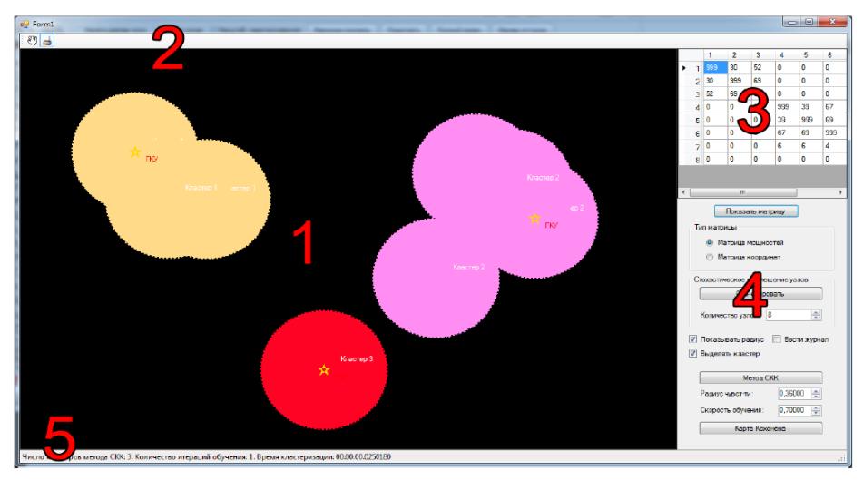
Figure 2 Software-modeling environment. The method of neural network clustering.
- 3. Radio visibility matrix for all network nodes.
- 4. Options panel consisting of the following elements: Matrix type selection: radio visibility matrix or coordinate matrix. Stochastic placement of nodes: setting the number of nodes that will be randomly placed on a twodimensional canvas. Show radius: displays the radius of the radio visibility
5. Status bar: Display of analytical clustering results, i.e. time and number of clusters.
Figure 3 shows the interface of the modeling environment for the matrix method of clustering.
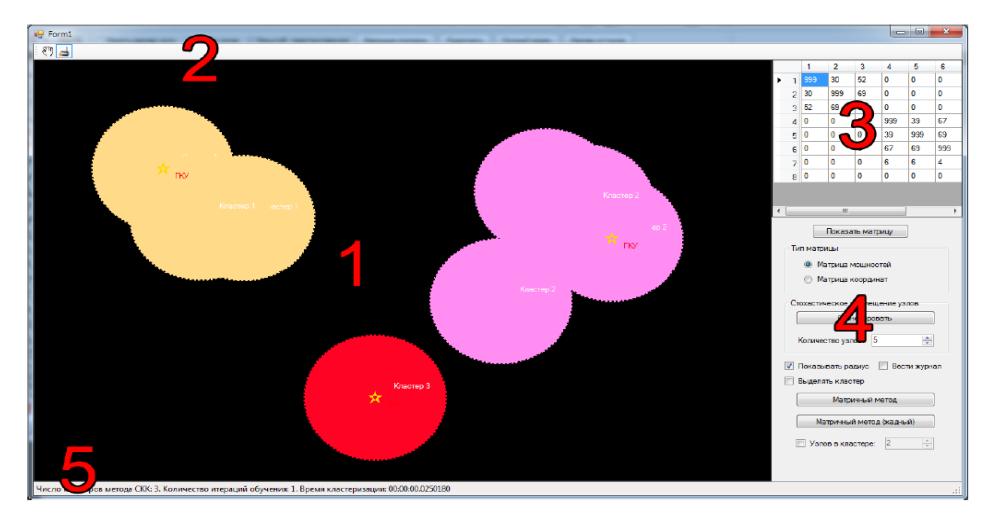
Figure 3 The interfaces of the modeling environment for the matrix method of clustering.
According to Figure 3, the elements marked by numbers coincide with Figure 2 with the exception of a part of the elements indicated by the number 4. Instead of the parameters of the previous clustering method, the control elements are presented for initiating the launch of the matrix clustering method with the ability to set an input parameter: the maximum number of nodes that can enter a cluster [20].
4.1 Modeling Method of Neural Network Clustering
Now, let us simulate the method of neural network clustering. As input, we will specify the number of nodes N and the radius of sensitivity of neurons R. The results will be a visual assessment of the quality of clustering and time t for which it was performed. Also, the number of formed clusters K will be known at the output.
Test number 1. Input parameters: N = 15; R = 0.26. Results: t = 0.045 seconds; K = 9. The visualization is shown in Figure 4.
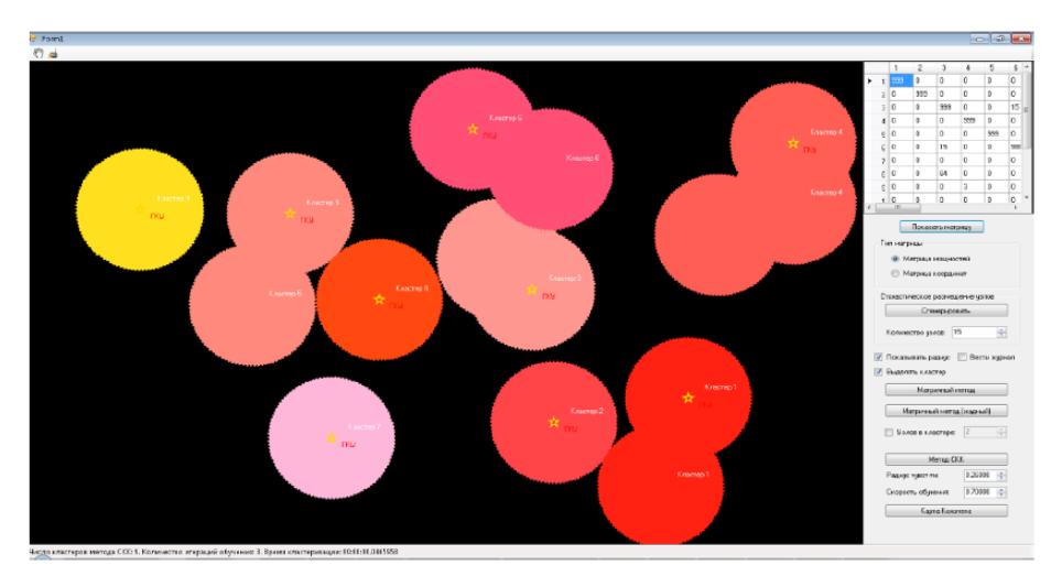
Figure 4 Test 1 – visualization of the results of the neural network clustering method.
Conclusion: intersecting nodes and nodes that are close to each other were combined into one cluster, isolated nodes entered their own separate cluster, respectively the set of neighbors for such nodes was empty ( ∈ ∅). The main cluster nodes (MCNs) of the clusters were allocated correctly [21].
Test number 2. Input parameters: N = 1000; R = 0.36. Results: t = 4 seconds; K = 17. The visualization is presented in Figure 5.
Conclusion: based on Figure 5 we see that visually clustering was done correctly; the clusters were selected; MCNs were identified. Only 4 seconds were spent on clustering 1000 nodes.
Test number 3. Input parameters: N = 1000; R = 0.22. Results: t = 20 minutes; K = 124. The visualization is presented in Figure 6.
Conclusion: with a decrease in R, the number of clusters increases, since the coverage radius for each cluster decreases. Therefore, the indication of a small R will allow for the formation of small-sized clusters.
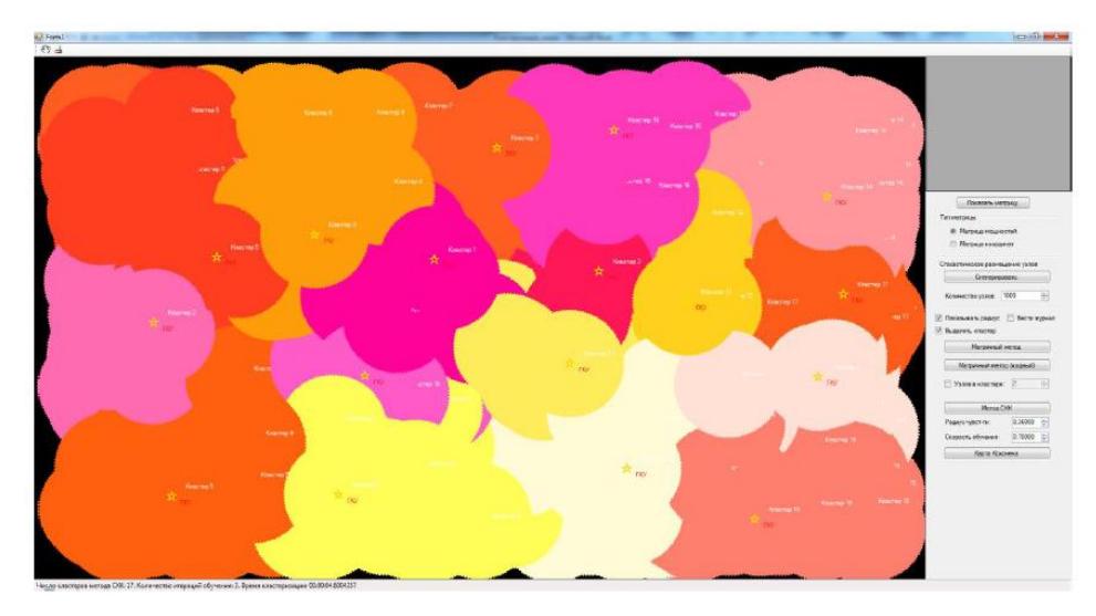
Figure 5 Test 2 – visualization of the results of the neural network clustering method.
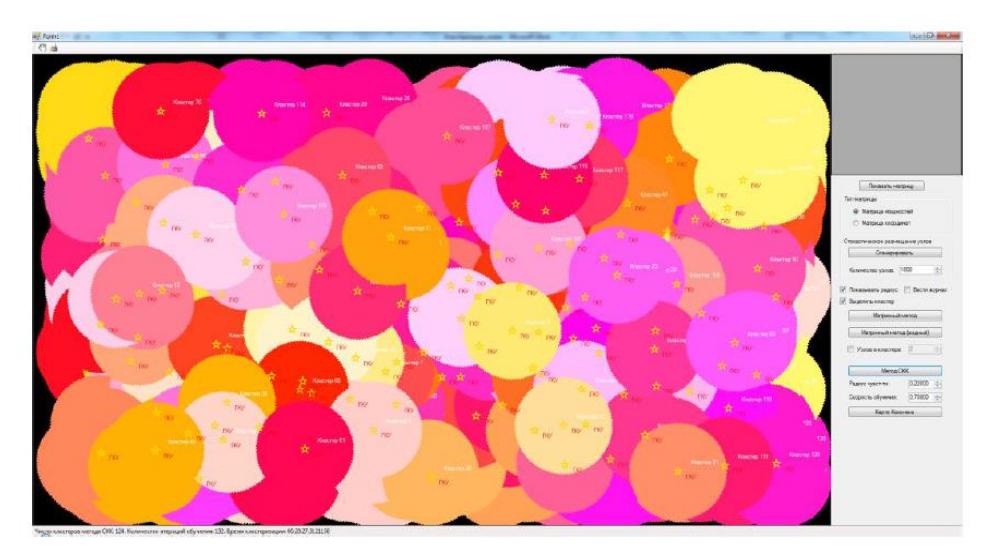
Figure 6 Test 3 – visualization of the results of the neural network clustering method.
Test number 4. Input parameters: N = 100; R = 0.36. Results: t = 0.23 seconds; K = 24. The visualization is presented in Figure 7.
Conclusion: the clusters were allocated correctly; isolated nodes and broken clusters were not observed; MCNs were allocated correctly.
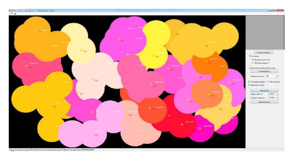
Figure 7 Test 4 – visualization of the results of the neural network clustering method.
4.2 Modeling the Matrix Method of Clustering
Now, let us model the matrix method of clustering. As input we set the number of nodes N and the number of nodes per cluster NK. The results, as in the previous paragraph, is a visual assessment of the quality of clustering and time t for which it was performed. We set the input parameters the same way as for the neural network clustering method [22].
Test number 1. Input parameters: N = 15; modification: no modifications. Results: t = 0.049 seconds; K = 10. The visualization is presented in Figure 8.
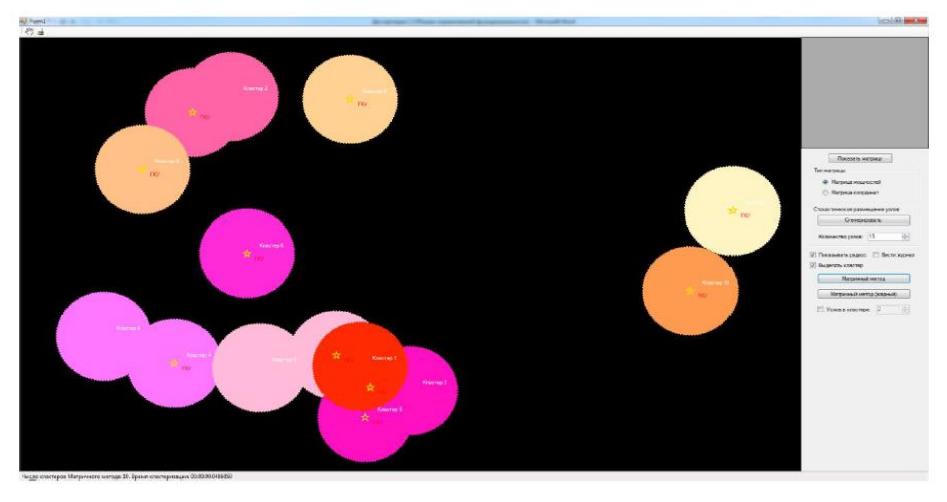
Figure 8 Test 1, visualization of the results of the matrix method of clustering.
Conclusion: visually, the clusters were selected correctly; MCNs in the cluster centers were also designated. Clustering used up more time in comparison with the method of neural network clustering by 0.016 seconds.
Test number 2. Input parameters: N = 1000; modification: greedy. Results: t = 43 seconds; K = 23. The visualization is presented in Figure 9.
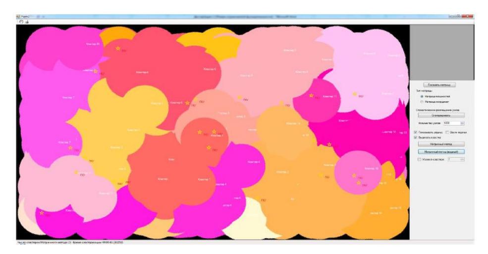
Figure 9 Test 2 – visualization of the results of the matrix (greedy) method of clustering.
Conclusion: visually, the clusters were formed correctly; MCNs were defined. Clustering was significantly longer in comparison with the method of neural network clustering with a radius of sensitivity of neurons R = 0.36. The difference was 39 seconds.
During the simulation, experiments were also performed with other clustering criteria: geographical coordinates of nodes and residual energy levels. As a result of the simulation, the network gave adequate clustering results. However, the level of residual energy should not be used as the only clustering parameter, since on the basis of this criterion it is impossible to determine how far the nodes are from each other and whether they can be within radio visibility of each other.
4.3 Comparison of Neural Network and Matrix Methods of Clustering Based on Modeling
During the simulation, visual results of clustering were obtained, which indicated that clustering was performed adequately according to the proposed methods. Moreover, it is important to note that in order to confirm the representativeness of the results, 300 additional tests for each method were performed. The observations obtained in these tests were approximately equal to the data obtained in the previous cases. Thus, the tests of the previous stage in the general case confirmed the dependencies revealed in the other experiments with this sample using a different set of values. Based on the experiments of the previous stage, we compiled the following summary table of clustering results.
| Input parameters | Output parameters | ||||
|---|---|---|---|---|---|
| N | R | Clustering method | t, seconds | K | Note |
| 15 | 0.26 | Neural network | 0.045 | 9 | Both methods worked correctly, but the |
| X | Matrix | 0.049 | 10 | neural network completed clustering a little faster | |
| 1000 | 0.36 | Neural network | 4 | 17 | Both methods worked correctly, but the |
| X | Matrix (greedy) | 43 | 23 | neural network method completed clustering much faster, the difference was 39 seconds | |
| 1000 | 0.22 | Neural network | 1200 | 124 | The matrix method worked faster, but |
| X | Matrix | 71 | 504 | cluster allocation was not energy efficient, the low speed of the neural network clustering method was due to the too low radius of sensitivity of the neurons, but, nevertheless the clusters were allocated energy-efficiently | |
| 100 | 0.36 | Neural network | 0.23 | 24 | Both methods worked correctly, but the |
| X | Matrix (greedy) | 0.33 | 15 | the neural network completed clustering a little faster | |
Table 2 Comparison of clustering results.
Based on Table 2 it can be seen that the neural network method is faster than the linear algorithm underlying the matrix clustering method. The speed of the method of neural network clustering depends on the radius of sensitivity of the neurons, which must be set in the range between 0.22 and 0.36. When setting a small value of R, we obtain a larger number of clusters and accordingly a smaller number of nodes will enter each cluster.
The clustering rate also depends on R, so clustering takes longer at small values. The value of R should be set small at low node density. At high node density, in contrast, the value must be set higher, depending on the desired cluster size. However, even if the setting of the average value of R is absolutely correct, it is still necessary to take into account the specifics of specific nodes and the desired cluster size.
The matrix method of clustering is inferior in speed to the method of neural network clustering and the standard version in most cases strongly splits the network into clusters, as a result of which the hierarchical structure energy efficiency decreases. The greedy modification of this method allows to allocate
clusters energy-efficiently, but is outperformed by the method of neural network clustering in terms of speed.
In most cases, the matrix method of clustering without modifications provides the same number of clusters at the output as the method of neural network clustering at R = 0.22. The same is true for the greedy modification of the matrix method and the method of neural network clustering at R close to 0.36. The neural network method allows to approximately set the cluster size and the matrix method allows to specify the maximum number of nodes that must be included in the cluster.
4.4 Modeling Routing Protocols
To evaluate the effectiveness of routing protocols in the BS, the metric of the network life cycle is used. This indicator can be estimated by modeling routing protocols. The simulation was performed in the environment of Math Works MATLAB R2014b. The program codes defining the logic of operation of the routing protocols LEACH, TEEN, GAF [8,11,17,18] in MATLAB operators (Figure 10) were taken from the official MathWorks website.
In the below protocol simulation codes, MATLAB adopted the well-known classical model of energy consumption in WSN, which was developed by a group of researchers led by W.R. Heinzelman. This model is based on the observation that the data transmission subsystems are the main energy consumers in WSN.
As input values for modeling each protocol routing we set the following initial conditions: size of touch field (for uniform random placement of wireless nodes): 100 x 100 meters; coordinates of the base station: x = 50; y = 50; number of wireless nodes: 100 pcs; size of the transmitted data packet: 4000 bits; initial energy E: 2 J. As a result of the simulation, the WSN life cycle was obtained under the control of the developed EDNCP protocol (energy distance neural clustering protocol) under the initial conditions, giving more than or equal to 1309 seconds (Figure 11).
The results of our comparative analysis revealed that the developed protocol is more effective than the others. The only disadvantage is the complexity of its implementation. EDNCP surpasses these protocols in features such as high scalability (over 10,000 nodes); independence of the protocol from the positioning modules (GPS/GLONAS); the ability to deliver packages from MCN to BS through intermediary nodes (other MCN or repeaters); the ability to use a mobile BS; the possibility of dynamic assignment of repeaters, which eliminates the dependence on certain nodes previously statically assigned as repeaters; accuracy of cluster formation.
Figure 10 Introduction to the MATLAB simulation code, indicating the use of the LEACH protocol code.
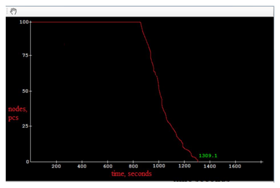
Figure 11 Graph of the ratio of the number of functioning nodes to time for the EDNCP protocol.
The advantages listed above indicate the effectiveness of using the EDNCP protocol in comparison with most well-known modern WSN routing protocols.
5 Conclusions
This paper presentsthe results of computer simulation of a solution for the routing problem in wireless sensor networks based on a neural mechanism by using neural network clustering, a matrix method for WSN clustering, and the protocol of energy distances of neural network clustering (EDNCP). The clustering methods were modeled in their own software-modeling environments written in a high-level programming language (C#) in the Microsoft Visual Studio 2010 software development environment. Based on computer modeling of the developed clustering methods it was revealed that the neural network clustering method had high efficiency on a variety of input data. In general, the tests were performed on 300 different input data sets, including placement of WSN nodes with different densities, different values of R and number of nodes N. Thus, at the output of the neural network clustering method you can get an energy-efficient hierarchical cluster structure, which can be used in WSN with a hierarchical data routing protocol.
The most famous routing protocols were simulated in MATLAB and compared with the developed routing protocol EDNCP according to the network life cycle metric. For comparison purposes the following protocols were selected: LEACH, TEEN, and GAF. It was found that the developed EDNCP protocol was 29% more efficient than the known analogues. An analysis of the effectiveness of the characteristics of the developed EDNCP protocol with known reference characteristics of the above protocols was performed. It was revealed that the developed EDNCP routing protocol has more efficient parameters than the known analogues. Based on the performed modeling and comparative analysis it was revealed that the developed EDNCP protocol allows the formation of clusters more accurately than the known analogues.